Simple scintillometry examples

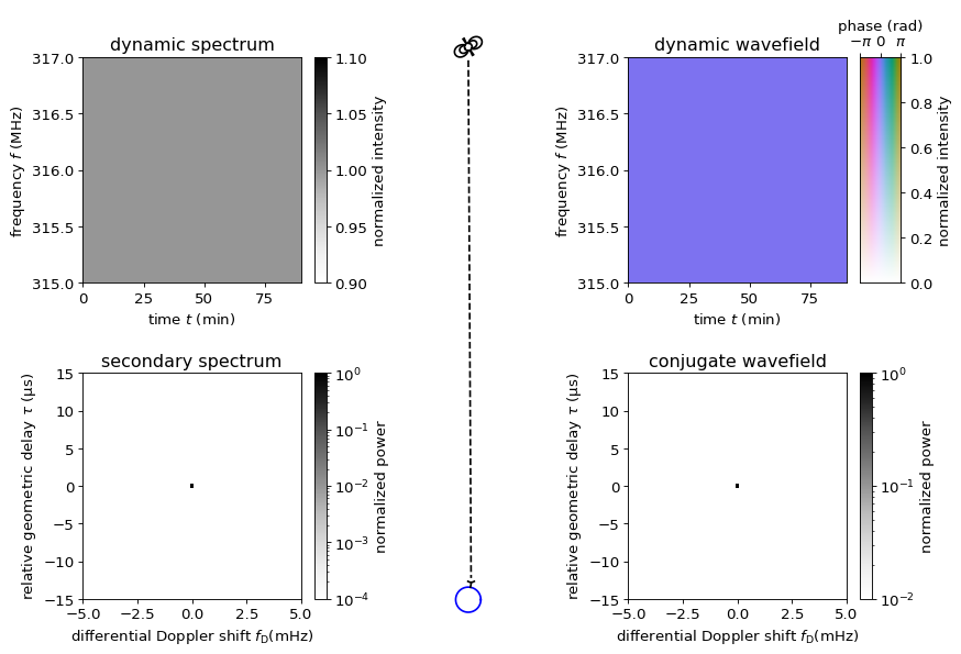
Consider observing a pulsar using a single radio dish. Let’s first assume that the pular is stationary. In this basic scenario, the pulsar’s radiation reaches the Earth via a direct line of sight, and the dynamic spectrum of the observation will look rather plain. In the secondary spectrum, there will be a single non-zero point at the origin.

A scattering screen

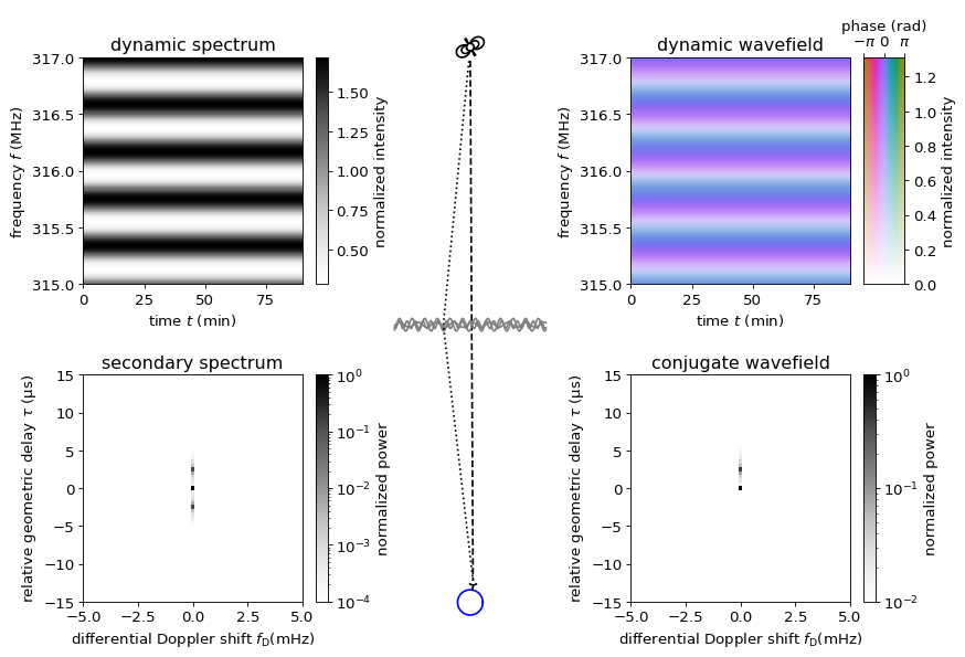
Now introduce a scattering screen somewhere in the space between the pulsar and Earth. This screen, a one-dimensional lens, will give rise to point-like scattering images of the pulsar. As a first step, we consider the effect of a single scattering image. In addition to the direct line of sight, there will now be a scattered beam via which radiation from the pulsar reaches Earth.

The radiation going via the scattered beam takes a longer path to Earth, and the resulting delay in arrival times between the two beams gives rise to an interference pattern in the dynamic spectrum. The interference pattern is stable in time (i.e., the dynamic spectrum is not really dynamic yet). In the secondary spectrum, two points show up along the vertical axis, corresponding to the relative geometric delay between the direct line of sight and the scattered beam. The reason there are two points, rather than one, is that the data (the interference pattern) do not distinguish which of the two images arrives first.

The effect of relative motion

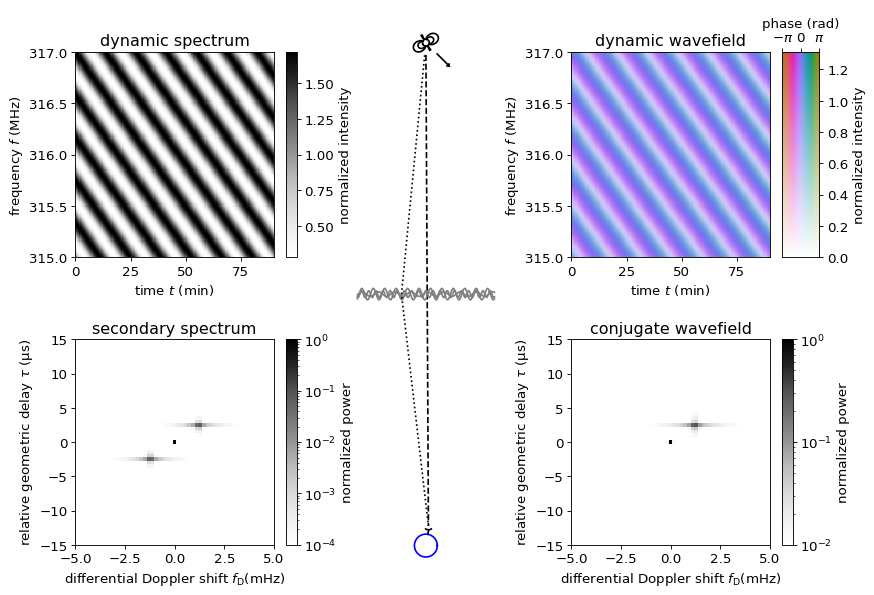
Until now we have assumed there is no relative motion between the pulsar, Earth, and the scattering screen (i.e., the interstellar medium). While in reality all these components will have their own space motion, they can all be included by a single effective velocity with which the line of sight moves with respect to the scattering screen.

This relative motion (represented in the schematic below by the arrow next to the pulsar) causes the delay between the two beams to change with time. As a result, the interference pattern resulting from their interaction shifts with time, seen as diagonal bands in the dynamic spectrum. In the secondary spectrum, the two points that were previously on the vertical axis have shifted to the differential Doppler shift corresponding to the effective velocity of the system.

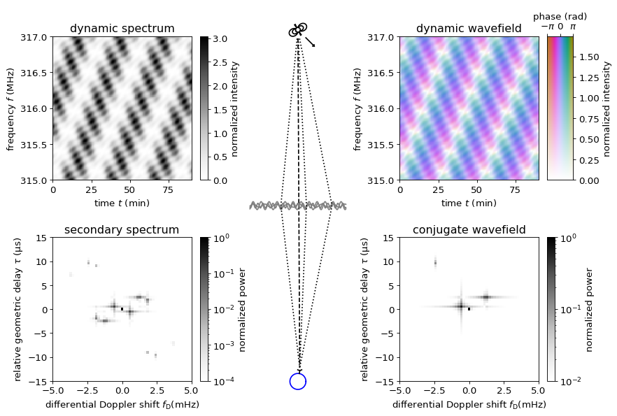
Two beams

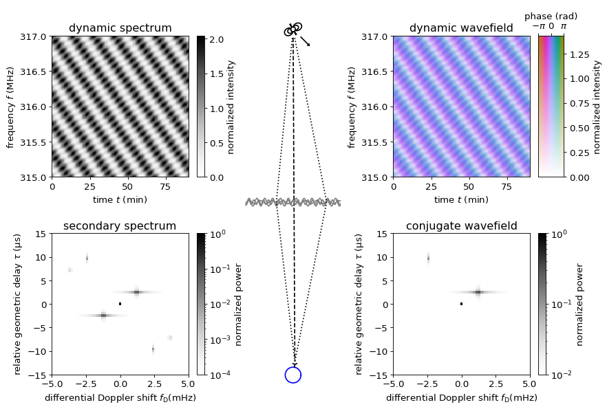
The lens will generally consist of many scattering points, each of which scatters an image of the pulsar in the direction of Earth. Now we consider what happens when the lens gives rise to two scattered beams. Each of these scattered beams will interact with the direct line-of-sight beam, causing its own interference pattern. In addition, the two scattered beams interact with one another, giving rise to a third interference pattern. Because the scattered images are generally much weaker than the direct one, the interference pattern due to their mutual interaction will be much weaker than those resulting from interaction of a scattered image and the direct one.

The dynamic spectrum is now a superposition of the three interference pattern (although the pattern due to the mutual interaction of the two scattered beams is too weak to discern in this example). In the secondary spectrum, four new points can be seen: two that correspond to the interaction of the new beam with the direct line-of-sight beam, and two weaker ones that correspond to the mutual interaction of the two scattered beams.

Three beams

Adding more beams further complicates the interference pattern.

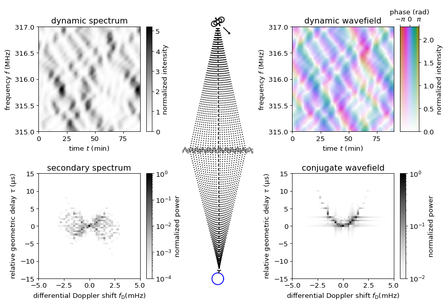
Many beams

When a relatively large number of beams is considered, the dynamic spectrum becomes so complex that the interference patterns due to individual pairs of beams can no longer been identified. It becomes more practical to characterize the dynamic spectrum as a pattern of bright (amplified) patches in time and frequency (known as “scintils”) against a less bright background.

In the secondary spectrum, the points arrising from interaction of a scattered image with the central one line up along parabolas with their extrema at the origin. The points caused by mutual interaction of scattered beams form “arclets”, inverted parabolas positioned along the main parabolas.

Note

For the purpose of generating simulated data in the examples shown here, we assume that the pulsars radio spectrum is flat and that there are no sources of noise in the observation. We use the following parameter values for the pulsar and the observation:

effective distance	\(d_\mathrm{eff}\)	0.5 kpc
effective proper motion	\(\mu_\mathrm{eff}\)	50 mas/yr
central observing frequency	\(f_\mathrm{obs}\)	316 MHz
bandpass	\(\Delta f\)	2 MHz
observation length	\(\Delta t\)	90 min
frequency channels	\(n_f\)	200
time bins	\(n_t\)	180