Scintillation velocities

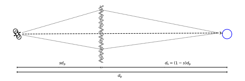
Consider a pulsar in a binary, observed through a single thin scattering screen that acts as a one-dimensional lens. The goal of these derivations is to examine how scintillometric measurements from Earth can constrain the physical parameters of the pulsar system and the screen.

Scintillometric observables

The basic scintillometric observable is the curvature \(\eta( t, \lambda )\) of the parabola in a secondary spectrum, taken at a reference time \(t\) and wavelength \(\lambda\). In terms of physical properties of the system, it can be expressed as

\[\eta = \frac{ \lambda^2 d_\mathrm{eff} }{ 2 c v_\mathrm{eff,\parallel}^2 },\]

where \(c\) is the speed of light, and \(d_\mathrm{eff}\) and \(v_\mathrm{eff,\parallel}\) are the effective distance and the effective velocity, respectively, to be defined below. Isolating the unknowns in this equation and taking the square root shows that curvature measurements constrain the quantity

\[\frac{ \lambda }{ \sqrt{ 2 c \eta } } = \frac{ \left| v_\mathrm{eff,\parallel} \right| } { \sqrt{ d_\mathrm{eff} } },\]

which we will refer to as the scaled effective velocity. This also shows that simultaneous curvature measurements taken at different wavelengths can be combined, leaving a time-series of scaled effective velocities as the relevant scintillometric observable to be modelled or fitted.

The effective distance

The distances from Earth to the pulsar and the scattering screen are denoted by \(d_\mathrm{p}\) and \(d_\mathrm{s}\), respectively. These two physical distances are combined into the effective distance

\[d_\mathrm{eff} = \frac{ d_\mathrm{p} d_\mathrm{s} } { d_\mathrm{p} - d_\mathrm{s} } = \frac{ 1 - s }{ s } d_\mathrm{p}.\]

Here, \(s\) is the fractional pulsar–screen distance (with \(0 \leq s \leq 1\)), given by

\[s = 1 - \frac{ d_\mathrm{s} }{ d_\mathrm{p} }.\]

The effective velocity

The scattering of the pulsar’s radiation by the screen gives rise to an interference pattern of bright and dark fringes in space. Because the pulsar, the screen, and Earth all move with respect to one another, an Earth-based observation will probe different points in this pattern over time.

The sky-plane velocity (i.e., the velocity component that is perpendicular to the direct line of sight) of the interference pattern relative to Earth, known as the effective velocity, is given by

\[\vec{v}_\mathrm{eff} = \frac{ 1 }{ s } \vec{v}_\mathrm{lens,sky} - \frac{ 1 - s }{ s } \vec{v}_\mathrm{p,sky} - \vec{v}_\mathrm{\oplus,sky}.\]

Here, \(\vec{v}_\mathrm{p,sky}\), \(\vec{v}_\mathrm{lens,sky}\), and \(\vec{v}_\mathrm{\oplus,sky}\) are the sky-plane velocities of the pulsar, the screen, and Earth, respectively, all generally specified relative to the Solar System’s barycentre. The pulsar’s sky-plane velocity can be split into a systemic component \(\vec{v}_\mathrm{p,sys,sky}\) (corresponding to the system’s proper motion), specified relative to the Solar System’s barycentre, and an orbital component \(\vec{v}_\mathrm{p,orb,sky}\), specified relative to the pulsar system’s barycentre: \(\vec{v}_\mathrm{p,sky} = \vec{v}_\mathrm{p,sys,sky} + \vec{v}_\mathrm{p,orb,sky}\).

Since we consider a one-dimensional lens, only velocity components parallel to the line of lensed images (marked by subscript ‘\(\parallel\)’ below) have any effect on the shift of the interference pattern. Thus, the equation for the effective velocity, considering only the relevant velocity components, becomes

\[v_\mathrm{eff,\parallel} = \frac{ 1 }{ s } v_\mathrm{lens,\parallel} - \frac{ 1 - s }{ s } v_\mathrm{p,\parallel} - v_{\oplus,\parallel}, \qquad \mathrm{with} \qquad v_\mathrm{p,\parallel} = v_\mathrm{p,sys,\parallel} + v_\mathrm{p,orb,\parallel}. \label{eq_v_eff} \tag{1}\]

In the following, we examine how the different velocities in equation \(\ref{eq_v_eff}\) that contribute to \(v_\mathrm{eff,\parallel}\) depend on the physical parameters of the pulsar system and the scattering screen. The first of these velocities, \(v_\mathrm{lens,\parallel}\), is a free parameter in the problem, leaving us to examine \(v_\mathrm{p,sys,\parallel}\), \(v_\mathrm{p,orb,\parallel}\) and \(v_{\oplus,\parallel}\).

The effective proper motion

It can sometimes be convenient to combine the effective distance and velocity into an effective proper motion

\[\vec{\mu}_\mathrm{eff} = \frac{ \vec{v}_\mathrm{eff} }{ d_\mathrm{eff} } = \vec{\mu}_\mathrm{lens} - \vec{\mu}_\mathrm{p} - \vec{\mu}_\oplus,\]

with

\[\vec{\mu}_\mathrm{lens} = \frac{ \vec{v}_\mathrm{lens,sky} }{ d_\mathrm{s} }, \qquad \vec{\mu}_\mathrm{p} = \frac{ \vec{v}_\mathrm{p,sky} }{ d_\mathrm{p} }, \qquad \vec{\mu}_\oplus = \frac{ \vec{v}_\mathrm{\oplus,sky} }{ d_\mathrm{eff} }.\]

Here, the pulsar’s proper motion consists of a systemic and an orbital component: \(\vec{\mu}_\mathrm{p} = \vec{\mu}_\mathrm{p,sys} + \vec{\mu}_\mathrm{p,orb}\), where the systemic component \(\vec{\mu}_\mathrm{p,sys}\) is often known from astrometric studies. As with the velocities, only proper motion components parallel to the line of lensed images are relevant:

\[\mu_\mathrm{eff,\parallel} = \mu_\mathrm{lens,\parallel} - \mu_\mathrm{p,\parallel} - \mu_{\oplus,\parallel}, \qquad \mathrm{with} \qquad \mu_\mathrm{p,\parallel} = \mu_\mathrm{p,sys,\parallel} + \mu_\mathrm{p,orb,\parallel}.\]

Finally, the effective proper motion relates to the scintillometric observables following

\[\frac{ \lambda }{ \sqrt{ 2 c \eta } } = \left| \mu_\mathrm{eff,\parallel} \right| \sqrt{ d_\mathrm{eff} }.\]

The pulsar’s systemic motion

The pulsar’s systemic velocity in the plane of the sky \(\vec{v}_\mathrm{p,sys,sky}\) can be found from the system’s proper motion \(\vec{\mu}_\mathrm{p,sys}\) following

\[\vec{v}_\mathrm{p,sys,sky} = d_\mathrm{p} \vec{\mu}_\mathrm{p,sys}.\]

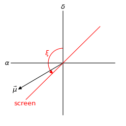
The component of this velocity that is parallel to the line of images formed by the lens is then given by

\[v_\mathrm{p,sys,\parallel} = d_\mathrm{p} \left[ \mu_\mathrm{p,sys,\alpha\ast} \sin( \xi ) + \mu_\mathrm{p,sys,\delta} \cos( \xi ) \right].\]

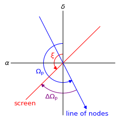
Here, \(\mu_\mathrm{p,sys,\alpha\ast}\) is proper motion’s right-ascension component (including the \(\cos( \delta_\mathrm{p} )\) term, with \(\delta_\mathrm{p}\) being the source’s declination), \(\mu_\mathrm{p,sys,\delta}\) is its declination component, and \(\xi\) is the position angle of the line of lensed images, measured from the celestial north through east, with \(0^\circ \leq \xi < 180^\circ\). Because the angle \(\xi\) is restricted to this range, it technically refers to the position angle of the eastern half of the line of lensed images.

The pulsar’s orbital motion – circular orbit

Let’s first consider the case of a pulsar in a circular orbit.

The \(xyz\) coordinate system and the orbital inclination

We introduce the right-handed orthonormal triad \((\hat{x}, \hat{y}, \hat{z})\) linked to the binary’s barycentre, with \(\hat{x}\) and \(\hat{y}\) in the plane of the sky, \(\hat{x}\) pointing to the pulsar’s ascending node (the point on the orbit that intersects the sky-plane, where the pulsar moves away from the observer), and \(\hat{z}\) pointing away from the observer. Since this is a right-handed coordinate system, if \(\hat{y}\) points upward as viewed by the observer, then \(\hat{x}\) points to the left (and the \(x\) coordinate increases towards the left).

The orbital inclination is parameterised by the angle \(i_\mathrm{p}\) between the direction towards the observer \(-\hat{z}\) and the binary’s orbital specific angular momentum \(\vec{h}_\mathrm{p} = \vec{r}_\mathrm{p} \times \vec{v}_\mathrm{p}\), where \(\vec{r}_\mathrm{p}\) and \(\vec{v}_\mathrm{p}\) denote the pulsar’s position and velocity, respectively. This angle is naturally restricted to the range \(0^\circ \le i_\mathrm{p} < 180^\circ\). As per the standard convention for orbits outside the Solar System, inclinations of \(i_\mathrm{p} < 90^\circ\) correspond to counterclockwise rotation on the sky and inclinations of \(i_\mathrm{p} > 90^\circ\) correspond to clockwise rotation on the sky, with \(i_\mathrm{p} = 90^\circ\) for an edge-on orbit (\(\vec{h}_\mathrm{p}\) anti-parallel to \(\hat{y}\)).

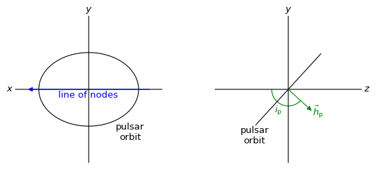
Left: observer’s view, looking in the direction of \(\hat{z}\). Right: side view, looking in the direction of \(\hat{x}\).

The pulsar’s position and velocity in \(xyz\) coordinates

In this \(xyz\) coordinate system, the pulsar’s position and velocity as function of the its orbital phase \(\phi_\mathrm{p} = 2 \pi ( t - t_\mathrm{asc,p} ) / P_\mathrm{orb,p}\), measured from the ascending node of the pulsar’s orbit, are given by

\[\begin{split}\vec{r}_\mathrm{p} = a_\mathrm{p} \left[ \begin{array}{r} \cos( \phi_\mathrm{p} ) \\ - \cos( i_\mathrm{p} ) \sin( \phi_\mathrm{p} ) \\ \sin( i_\mathrm{p} ) \sin( \phi_\mathrm{p} ) \end{array} \right], \qquad \vec{v}_\mathrm{p} = v_\mathrm{0,p} \left[ \begin{array}{r} - \sin( \phi_\mathrm{p} ) \\ - \cos( i_\mathrm{p} ) \cos( \phi_\mathrm{p} ) \\ \sin( i_\mathrm{p} ) \cos( \phi_\mathrm{p} ) \end{array} \right].\end{split}\]

Here, \(t_\mathrm{asc,p}\) is the pulsar’s time of ascending node passage, \(P_\mathrm{orb,p}\) is the binary’s orbital period, \(a_\mathrm{p}\) is the semi-major axis of the pulsar’s orbit, and \(v_\mathrm{0,p} = 2 \pi a_\mathrm{p} / P_\mathrm{orb,p}\) is the mean orbital speed of the pulsar. Pulsar timing studies normally constrain \(t_\mathrm{asc,p}\) and \(P_\mathrm{orb,p}\), as well as the pulsar orbit’s projected semi-major axis \(a_\mathrm{p} \sin( i_\mathrm{p} )\) and hence the pulsar’s radial-velocity amplitude \(K_\mathrm{p} = v_\mathrm{0,p} \sin( i_\mathrm{p} ) = 2 \pi a_\mathrm{p} \sin( i_\mathrm{p} ) / P_\mathrm{orb,p}\).

The orbit’s orientation on the sky and the sky-plane velocity

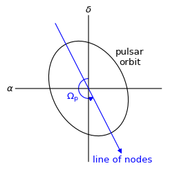
The orientation of the pulsar’s orbit on the sky is parameterised by its longitude of ascending node \(\Omega_\mathrm{p}\), measured from the celestial north through east.

In the equatorial coordinate system, the pulsar’s orbital sky-plane velocity is \(\vec{v}_\mathrm{p,orb,sky} = (v_\mathrm{p,\alpha\ast}, v_\mathrm{p,\delta}, 0)\) with

\[\begin{split}v_\mathrm{p,\alpha\ast} &= \vec{v}_\mathrm{p} \cdot \hat{\alpha} = - v_\mathrm{0,p} \left[ \sin( \Omega_\mathrm{p} ) \sin( \phi_\mathrm{p} ) - \cos( \Omega_\mathrm{p} ) \cos( i_\mathrm{p} ) \cos( \phi_\mathrm{p} ) \right], \\ v_\mathrm{p,\delta} &= \vec{v}_\mathrm{p} \cdot \hat{\delta} = - v_\mathrm{0,p} \left[ \cos( \Omega_\mathrm{p} ) \sin( \phi_\mathrm{p} ) + \sin( \Omega_\mathrm{p} ) \cos( i_\mathrm{p} ) \cos( \phi_\mathrm{p} ) \right].\end{split}\]

Projecting the sky-plane velocity onto the line of lensed images

The component of the pulsar’s orbital sky-plane velocity \(\vec{v}_\mathrm{p,orb,sky}\) that is parallel to the line of images formed by the lens is then given by

\[\begin{split}\begin{align} v_\mathrm{p,orb,\parallel} &= v_\mathrm{p,\alpha\ast} \sin( \xi ) + v_\mathrm{p,\delta} \cos( \xi ) \\ &= - v_\mathrm{0,p} \left[ \cos( \Delta\Omega_\mathrm{p} ) \sin( \phi_\mathrm{p} ) - \sin( \Delta\Omega_\mathrm{p} ) \cos( i_\mathrm{p} ) \cos( \phi_\mathrm{p} ) \right]. \label{eq_v_p_orb_parallel} \tag{2} \end{align}\end{split}\]

where \(\Delta\Omega_\mathrm{p} = \xi - \Omega_\mathrm{p}\) is the angle of the line of lensed images measured from the ascending node of the pulsar orbit.

The velocity modulation’s amplitude and phase offset

Equation \(\ref{eq_v_p_orb_parallel}\) for the pulsar’s orbital sky-plane velocity’s screen component \(v_\mathrm{p,orb,\parallel}\) describes a sinusoid as a function of orbital phase \(\phi_\mathrm{p}\). Via some trigonometry, this equation can be rewritten as

\[v_\mathrm{p,orb,\parallel} = - v_\mathrm{0,p} b_\mathrm{p} \sin( \phi_\mathrm{p} - \chi_\mathrm{p} ) = - \frac{ K_\mathrm{p} }{ \sin( i_\mathrm{p} ) } b_\mathrm{p} \sin( \phi_\mathrm{p} - \chi_\mathrm{p} ).\]

The sinusoid’s phase offset \(\chi_\mathrm{p}\) conforms to the relations

\[\cos( \chi_\mathrm{p} ) = \frac { \cos( \Delta\Omega_\mathrm{p} ) }{ b_\mathrm{p} } \qquad \mathrm{and} \qquad \sin( \chi_\mathrm{p} ) = \frac{ \sin( \Delta\Omega_\mathrm{p} ) \cos( i_\mathrm{p} ) } { b_\mathrm{p} }.\]

Using the 2-argument arctangent function \(\DeclareMathOperator{\arctantwo}{arctan2} \arctantwo(y, x)\), these can be combined into

\[\chi_\mathrm{p} = \arctantwo \left[ \sin( \Delta\Omega_\mathrm{p} ) \cos( i_\mathrm{p} ), \cos( \Delta\Omega_\mathrm{p} ) \right].\]

The parameter \(b_\mathrm{p}\) modifying the sinusoid’s amplitude (with \(0 \leq b_\mathrm{p} \leq 1\)) is given by

\[b_\mathrm{p}^2 = \cos^2( \Delta\Omega_\mathrm{p} ) + \sin^2( \Delta\Omega_\mathrm{p} ) \cos^2( i_\mathrm{p} ) = \frac{ 1 - \sin^2( i_\mathrm{p} ) } { 1 - \sin^2( i_\mathrm{p} ) \cos^2( \chi_\mathrm{p} ) }.\]

Earth’s motion around the Sun

Earth’s velocity projected onto the line of lensed images

Earth’s sky-plane velocity \(\vec{v}_\mathrm{\oplus,sky}\) is its velocity, relative to the Solar System’s barycentre, in the plane perpendicular to the line of sight towards the source. It can be found in the same way as the pulsar’s orbital sky-plane velocity \(\vec{v}_\mathrm{p,orb,sky}\), using an \(xyz\) coordinate system with the same orientation, but linked to the Solar System’s barycentre, and substituting the subscript ‘\(\mathrm{p}\)’ with the subscript ‘\(\oplus\)’ in the above derivations. Thus, under the simplifying assumption that Earth’s orbit around the Solar System’s barycentre is circular, the component of Earth’s sky-plane velocity along the line of lensed images is given by

\[v_{\oplus,\parallel} = - v_{0,\oplus} b_\oplus \sin( \phi_\oplus - \chi_\oplus ),\]

with

\[v_{0,\oplus} = \frac{ 2 \pi a_\oplus }{ P_\mathrm{orb,\oplus} }, \qquad b_\oplus^2 = \frac{ 1 - \sin^2( i_\oplus ) } { 1 - \sin^2( i_\oplus ) \cos^2( \chi_\oplus ) }, \qquad \phi_\oplus = 2 \pi \frac{ t - t_\mathrm{asc,\oplus} } { P_\mathrm{orb,\oplus} },\]

\[\chi_\oplus = \arctantwo \left[ \sin( \Delta\Omega_\oplus ) \cos( i_\oplus ), \cos( \Delta\Omega_\oplus ) \right], \qquad \Delta\Omega_\oplus = \xi - \Omega_\oplus.\]

Earth’s orbital orientation

In contrast to the pulsar, all of Earth’s orbital parameters (\(P_\mathrm{orb,\oplus}\), \(a_\oplus\), \(i_\oplus\), \(\Omega_\oplus\), \(t_\mathrm{asc,\oplus}\)) are known. The orientation of Earth’s orbit with respect to the line of sight, parameterised by \(i_\oplus\) and \(\Omega_\oplus\), can be derived from the pulsar system’s ecliptic coordinates \((\lambda_\mathrm{p}, \beta_\mathrm{p})\).

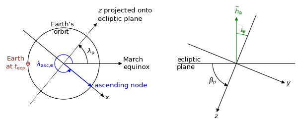
Left: top-down view, looking in the direction of \(-\vec{h}_\oplus\). Right: side view, looking in the direction of \(\hat{x}\).

The inclination of Earth’s orbital plane with respect to the line of sight \(i_\oplus\) is defined in the same way as the pulsar’s orbital inclination: it is the angle between the \(-\hat{z}\) axis (pointing from the Solar System’s barycentre to the direction opposite of the pulsar) and the Earth’s orbital specific angular momentum vector \(\vec{h}_\oplus\). It is given by

\[i_\oplus = \beta_\mathrm{p} + 90^\circ.\]

The restriction on the pulsar’s ecliptic latitude \(-90^\circ \le \beta_\mathrm{p} \le 90^\circ\) leads to the expected range of allowed inclinations \(0^\circ \le i_\oplus \le 180^\circ\). The convention for the sense of rotation is also the same: \(i_\oplus < 90^\circ\) for counterclockwise rotation when viewing in the \(\hat{z}\) direction and \(i_\oplus > 90^\circ\) for clockwise rotation.

Earth’s ascending node with respect to the line of sight is the point on the orbit where Earth passes through the observing plane in the direction of the pulsar. In this context, the longitude of ascending node \(\Omega_\oplus\) is equivalent to the position angle of Earth’s ascending node with respect to the coordinates of the pulsar system:

\[\Omega_\oplus = \mathcal{P}( X_\mathrm{p}, X_\mathrm{asc,\oplus} ).\]

Here, \(\mathcal{P}( X_1, X_2 )\) yields the position angle (east of north) from position \(X_1\) to position \(X_2\) (for details on this computation, see, e.g., the Wikipedia article on position angle), \(X_\mathrm{p} = (\alpha_\mathrm{p}, \delta_\mathrm{p})\) denotes the equatorial coordinates of the pulsar system, and \(X_\mathrm{asc,\oplus} = (\alpha_\mathrm{asc,\oplus}, \delta_\mathrm{asc,\oplus})\) is the equatorial coordinates of Earth’s ascending node. The latter can be found from its ecliptic coordinates \((\lambda_\mathrm{asc,\oplus}, \beta_\mathrm{asc,\oplus}) = (\lambda_\mathrm{p} - 90^\circ, 0)\).

Finally, under the simplifying assumption that Earth’s orbit is circular, the time of Earth’s passage through the ascending node is given by

\[t_\mathrm{asc,\oplus} = t_\mathrm{eqx} + P_\mathrm{orb,\oplus} \frac{ \lambda_\mathrm{p} + 90^\circ }{ 360^\circ },\]

where \(t_\mathrm{eqx}\) is the time of the March equinox.

Combining the lens, pulsar, and Earth terms

Combining the different terms in equation \(\ref{eq_v_eff}\) contributing to \(v_\mathrm{eff,\parallel}\) gives

\[v_\mathrm{eff,\parallel} = \underbrace{ \frac{ 1 }{ s } v_\mathrm{lens,\parallel} }_\textrm{lens motion} - \underbrace{ \frac{ 1 - s }{ s } d_\mathrm{p} \left[ \mu_\mathrm{p,sys,\alpha\ast} \sin( \xi ) + \mu_\mathrm{p,sys,\delta} \cos( \xi ) \right] }_\textrm{pulsar's systemic motion} + \underbrace{ \frac{ 1 - s }{ s } v_\mathrm{0,p} b_\mathrm{p} \sin( \phi_\mathrm{p} - \chi_\mathrm{p} ) }_\textrm{pulsar's orbital motion} + \underbrace{ \vphantom{ \frac{ 1 }{ s } } v_{0,\oplus} b_\oplus \sin( \phi_\oplus - \chi_\oplus ) }_\textrm{Earth's orbital motion}.\]

Filling in the terms for effective proper motion gives

\[\mu_\mathrm{eff,\parallel} = \underbrace{ \vphantom{ \frac{ v_\mathrm{0,p} }{ d_\mathrm{p} } } \frac{ v_\mathrm{lens,\parallel} }{ d_\mathrm{s} } }_\textrm{lens motion} - \underbrace{ \vphantom{ \frac{ v_\mathrm{0,p} }{ d_\mathrm{p} } } \left[ \mu_\mathrm{p,sys,\alpha\ast} \sin( \xi ) + \mu_\mathrm{p,sys,\delta} \cos( \xi ) \right] }_\textrm{pulsar's systemic motion} + \underbrace{ \frac{ v_\mathrm{0,p} }{ d_\mathrm{p} } b_\mathrm{p} \sin( \phi_\mathrm{p} - \chi_\mathrm{p} ) }_\textrm{pulsar's orbital motion} + \underbrace{ \vphantom{ \frac{ v_\mathrm{0,p} }{ d_\mathrm{p} } } \frac{ v_{0,\oplus} }{ d_\mathrm{eff} } b_\oplus \sin( \phi_\oplus - \chi_\oplus ) }_\textrm{Earth's orbital motion}.\]

This shows that the scaled effective velocity can be written as the normed sum of two sinusoids and a constant offset:

\[\frac{ \left| v_\mathrm{eff,\parallel} \right| }{ \sqrt{ d_\mathrm{eff} } } = \left| \mu_\mathrm{eff,\parallel} \right| \sqrt{ d_\mathrm{eff} } = \left| A_\oplus \sin( \phi_\oplus - \chi_\oplus ) + A_\mathrm{p} \sin( \phi_\mathrm{p} - \chi_\mathrm{p} ) + C \right|,\]

with

\[\begin{split}A_\oplus &= \frac{ v_{0,\oplus} }{ \sqrt{ d_\mathrm{eff} } } b_\oplus = \frac{ 1 }{ \sqrt{ d_\mathrm{eff} } } \frac{ 2 \pi a_\oplus }{ P_\mathrm{orb,\oplus} } b_\oplus, \\[1em] A_\mathrm{p} &= \frac{ 1 - s }{ s } \frac{ v_\mathrm{0,p} }{ \sqrt{ d_\mathrm{eff} } } b_\mathrm{p} = \frac{ \sqrt{ d_\mathrm{eff} } }{ d_\mathrm{p} } \frac{ K_\mathrm{p} }{ \sin( i_\mathrm{p} ) } b_\mathrm{p}, \\[1em] C &= \frac{ 1 }{ s } \frac{ v_\mathrm{lens,\parallel} }{ \sqrt{ d_\mathrm{eff} } } - \frac{ 1 - s }{ s } \frac{ v_\mathrm{p,sys,\parallel} }{ \sqrt{ d_\mathrm{eff} } } = \frac{ 1 }{ s } \frac{ v_\mathrm{lens,\parallel} }{ \sqrt{ d_\mathrm{eff} } } - \sqrt{ d_\mathrm{eff} } \left[ \mu_\mathrm{p,sys,\alpha\ast} \sin( \xi ) + \mu_\mathrm{p,sys,\delta} \cos( \xi ) \right].\end{split}\]