Different transforms for constructing secondary spectra
Usually, the secondary spectrum is constructed from a straight FFT of the
dynamic spectrum. For wide bandwidths, this leads to smearing, making the
structure of arcs and inverted arclets less clear. This tutorial shows how
one can use the screens.conjspec.ConjugateSpectrum class to
create so-called nu-t transforms, where the time axis is replaced by one that
has time scaled with frequency. It also shows how another technique that is
sometimes used, in which the frequency axis is replaced by one in wavelength,
produces a sharp arc, but smears any arclets.
The combined codeblocks in this tutorial can be downloaded as a Python script and as a Jupyter notebook:
- Python script:
- Jupyter notebook:
Preliminaries
Start with some standard imports and a handy function for presenting images.
import numpy as np
import matplotlib.pyplot as plt
import astropy.units as u
import astropy.constants as const
from astropy.visualization import quantity_support
from scipy.signal.windows import tukey
from screens.fields import dynamic_field
from screens.dynspec import DynamicSpectrum as DS
from screens.conjspec import ConjugateSpectrum as CS
from screens.visualization import axis_extent
Set up a scattering screen
We create a weakly modulated scattering screen with many faint images, as well as, to show the effect of different transforms, one brighter image (leading to one arclet), and a small gap.
sig = 0.3*u.mas
theta = np.linspace(-1, 1, 28*16, endpoint=False) << u.mas
a = 0.01 * np.exp(-0.5*(theta/sig)**2).to_value(u.one)
realization = a * np.exp(2j*np.pi*np.random.uniform(size=theta.shape))
realization[4*16] = 0.03  # A bright spot
realization[-5*16:-5*16+8] = 0  # A small gap
realization[np.where(theta == 0)] = 1  # Make line of sight bright
# Normalize
realization /= np.sqrt((np.abs(realization)**2).sum())
# Plot amplitude as a function of theta
plt.figure(figsize=(12., 3.))
plt.semilogy(theta, np.abs(realization), '+')
plt.xlabel(r"$\theta\ (mas)$")
plt.ylabel("A")
plt.show()

Create standard dynamic and secondary spectra
Now make a (tapered) dynamic spectrum and the regular secondary spectrum. One sees how badly smeared the signal is.
# Observation parameters
fobs = 1320. * u.MHz
d_eff = 0.25 * u.kpc
mu_eff = 100 * u.mas / u.yr
# Frequency and time grids
f = fobs + np.linspace(-250*u.MHz, 250*u.MHz, 400, endpoint=False)
t = np.linspace(-150*u.minute, 150*u.minute, 200, endpoint=False)[:, np.newaxis]

# Calculate dynamic spectrum, adding some Gaussian noise.
dynspec = np.abs(dynamic_field(theta, 0., realization, d_eff, mu_eff, f, t).sum(0))**2
noise = 0.02
dynspec += noise * np.random.normal(size=dynspec.shape)
# Normalize
dynspec /= dynspec.mean()
# Smooth edges to reduce peakiness in sec. spectrum.
alpha_nu = 0.25
alpha_t = 0.5  # Bit larger so nu-t transform also is OK.
taper = (tukey(dynspec.shape[-1], alpha=alpha_nu)
         * tukey(dynspec.shape[0], alpha=alpha_t)[:, np.newaxis])
dynspec = (dynspec - 1.0) * taper + 1.0
# Create Dynamic and Conjugate spectra.
ds = DS(dynspec, f=f, t=t, noise=noise)
cs = CS.from_dynamic_spectrum(ds)
cs.tau <<= u.us  # nicer than 1/MHz
cs.fd <<= u.mHz  # nicer than 1/min

plt.figure(figsize=(12, 8.))
plt.subplot(121)
plt.imshow(ds.dynspec.T, origin='lower', aspect='auto',
           extent=axis_extent(ds.t, ds.f), cmap='Greys')
plt.xlabel(rf"$t\ ({ds.t.unit.to_string('latex')[1:-1]})$")
plt.ylabel(rf"$f\ ({ds.f.unit.to_string('latex')[1:-1]})$")
plt.title(rf"$\nu - t$")
plt.colorbar()

plt.subplot(122)
plt.imshow(np.log10(cs.secspec.T), origin='lower', aspect='auto',
           extent=axis_extent(cs.fd, cs.tau), cmap='Greys', vmin=-9, vmax=-2)
plt.xlabel(rf"$f_{{D}}\ ({cs.fd.unit.to_string('latex')[1:-1]})$")
plt.ylabel(rf"$\tau\ ({cs.tau.unit.to_string('latex')[1:-1]})$")
plt.colorbar()
plt.show()

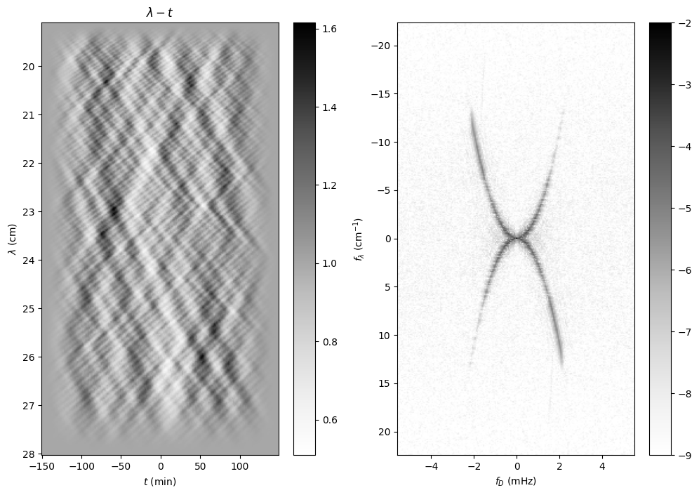
Try a wavelength transform
Replacing the frequency axis by one constant in wavelength leads to a much clearer main arc, but the arclet or hole can still not be seen.
# Rebin frequency to wavelength.
w = np.linspace(const.c / f[0], const.c / f[-1], f.shape[-1]).to(u.cm)
dw = w[1] - w[0]
_ds = np.stack([np.interp(const.c/w, f, _d) for _d in dynspec])
ds_w = DS(_ds, f=w, t=t, noise=noise)
# And turn it into a secondary spectrum (straight FT)
cs_w = CS.from_dynamic_spectrum(ds_w)
cs_w.fd <<= u.mHz
dfl = cs_w.tau[1] - cs_w.tau[0]

plt.figure(figsize=(12, 8.))
plt.subplot(121)
plt.imshow(ds_w.dynspec.T, origin='lower', aspect='auto',
           extent=axis_extent(ds_w.t, ds_w.f), cmap='Greys')
plt.xlabel(rf"$t\ ({ds_w.t.unit.to_string('latex')[1:-1]})$")
plt.ylabel(rf"$\lambda\ ({ds_w.f.unit.to_string('latex')[1:-1]})$")
plt.title(rf"$\lambda - t$")
plt.colorbar()

plt.subplot(122)
plt.imshow(np.log10(cs_w.secspec.T), origin='lower', aspect='auto',
           extent=axis_extent(cs_w.fd, cs_w.tau), cmap='Greys', vmin=-9, vmax=-2)
plt.xlabel(rf"$f_{{D}}\ ({cs_w.fd.unit.to_string('latex')[1:-1]})$")
plt.ylabel(rf"$f_{{\lambda}}\ ({cs_w.tau.unit.to_string('latex_inline')[1:-1]})$")
plt.colorbar()
plt.show()
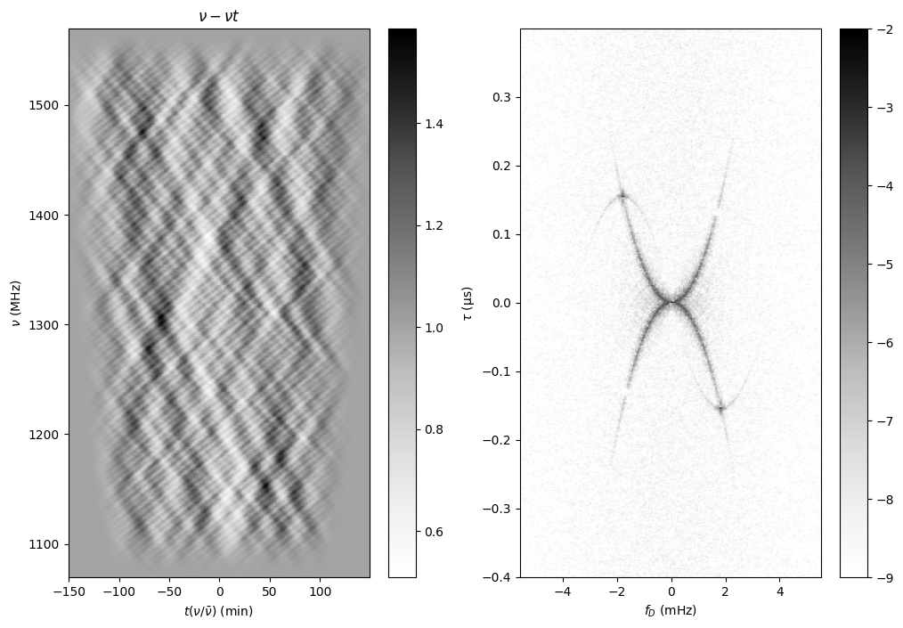
The amazing nu-t transform
The nu-t transform [1], in which one replaces the time axis with one scaled by frequency, brings out both the main arc, the arclet, and the gap.
# Rebin time to t / f so it becomes a nu t transform
tt = t * f.mean() / f
_ds = np.stack([np.interp(_t, t[:, 0], _d) for _t, _d in zip(tt.T, dynspec.T)]).T
ds_t = DS(_ds, f=f, t=t, noise=noise)

nut = CS.from_dynamic_spectrum(ds_t)
nut.tau <<= u.us
nut.fd <<= u.mHz

plt.figure(figsize=(12, 8.))
plt.subplot(121)
plt.imshow(ds_t.dynspec.T, origin='lower', aspect='auto',
           extent=axis_extent(ds_t.t, ds_t.f), cmap='Greys')
plt.xlabel(rf"$t(\nu/\bar{{\nu}})\ ({ds_t.t.unit.to_string('latex')[1:-1]})$")
plt.ylabel(rf"$\nu\ ({ds_t.f.unit.to_string('latex')[1:-1]})$")
plt.title(rf"$\nu - \nu t$")
plt.colorbar()

plt.subplot(122)
plt.imshow(np.log10(nut.secspec.T), origin='lower', aspect='auto',
           extent=axis_extent(nut.fd, nut.tau), cmap='Greys', vmin=-9, vmax=-2)
plt.xlabel(rf"$f_{{D}}\ ({nut.fd.unit.to_string('latex')[1:-1]})$")
plt.ylabel(rf"$\tau\ ({nut.tau.unit.to_string('latex')[1:-1]})$")
plt.colorbar()
plt.show()
One does not actually have to rebin to do the nu-t transform, but one
can instead pass in scaled times to the
from_dynamic_spectrum() method,
as follows (note: passing in scaled frequencies is not yet possible).
nut2 = CS.from_dynamic_spectrum(dynspec, f=f, t=t*f/f.mean(), fd=nut.fd[:, 0])
nut2.tau <<= u.us
# Show new one
plt.figure(figsize=(12, 8.))
plt.subplot(121)
plt.imshow(np.log10(nut2.secspec.T), origin='lower', aspect='auto',
           extent=axis_extent(nut2.fd, nut2.tau), cmap='Greys', vmin=-9, vmax=-2)
plt.xlabel(rf"$f_{{D}}\ ({nut2.fd.unit.to_string('latex')[1:-1]})$")
plt.ylabel(rf"$\tau\ ({nut2.tau.unit.to_string('latex')[1:-1]})$")
plt.title("From regular dynamic spectrum with scaled times.")
plt.colorbar()
# and compare with one from rebinned dynamic spectrum.
plt.subplot(122)
plt.imshow(np.log10(nut.secspec.T), origin='lower', aspect='auto',
           extent=axis_extent(nut.fd, nut.tau), cmap='Greys', vmin=-9, vmax=-2)
plt.xlabel(rf"$f_{{D}}\ ({nut.fd.unit.to_string('latex')[1:-1]})$")
plt.ylabel(rf"$\tau\ ({nut.tau.unit.to_string('latex')[1:-1]})$")
plt.title("From rebinned dynamic spectrum.")
plt.colorbar()
plt.show()
