Using the Screen1D class
This tutorial describes how to generate synthetic data corresponding to a
single-dish observation of a pulsar whose radiation is scattered by a single
one-dimensional screen. It explains how to use the screens.screen
module, in particular its Screen1D class and the
observe() method, to quickly set up a
one-dimensional scattering screen and generate synthetic observations of the
pulsar through such a screen.
The combined codeblocks in this tutorial can be downloaded as a Python script and as a Jupyter notebook:
- Python script:
- Jupyter notebook:
Preliminaries
Imports.
import numpy as np
import matplotlib.pyplot as plt
from matplotlib.colors import LogNorm

from astropy import units as u
from astropy.coordinates import (
    CartesianRepresentation, CylindricalRepresentation,
    UnitSphericalRepresentation)

from screens.screen import Source, Screen1D, Telescope
from screens.fields import phasor
# A handy function to create extents to use with imshow.
from screens.visualization import axis_extent
Construct the system’s components
The screens.screen module lets us first define the components of the
scintillometry system (pulsar, scattering screen, and telescope) and consider
their interaction afterwards.
For this simple example, we will use a reference frame whose \(z\)-axis points along the direct line of sight from Earth to the pulsar, and we will assume that the scattering screen and Earth are at rest in this reference frame. Although not yet necessary for defining the individual components, let’s already set the distances (from Earth) to the pulsar \(d_\mathrm{p}\) and to the screen \(d_\mathrm{s}\).
d_p = 0.5 * u.kpc
d_s = 0.25 * u.kpc
The pulsar
Create the pulsar using the Source class. Its
three-dimensional position and velocity vectors, pos and vel, need to
be given as Asropy CartesianRepresentation
objects. By default, the position is zero. Note that this position does not
include the distance; the Source object only
defines the properties of the source and could in principle be observed from
anywhere. The (scaled) brightness of the pulsar can be set using the
magnification attribute; by default, this attribute is set to unity.
pulsar_vel = CartesianRepresentation(-300., 0., 0., unit=u.km/u.s)

pulsar = Source(vel=pulsar_vel)

print(pulsar)
<Source
    pos=(0., 0., 0.) AU,
    vel=(-300., 0., 0.) km / s,
    magnification=1.0>
The scattering screen
Create the scattering screen using the Screen1D
class with the following arguments:
The unit normal vector
normalthat defines the orientation of the screen. It points in the direction of the line of images formed by the screen and it is perpendicular to the direct line of sight from Earth to the pulsar. This should be an AstropyCartesianRepresentationobject. Here, we use Astropy’sCylindricalRepresentationclass to create the unit vector in the \(xy\)-plane of the reference frame (with the azimuth measured counterclockwise from the \(x\)-axis), and convert it to aCartesianRepresentationobject using theto_cartesian()method.The positions
pof the lensed images along the line defined bynormal, given as an AstropyQuantityobject.The velocities
vof the images along that line (in this case all images have the same velocity, zero).The array
magnificationcontaining the complex magnifications of the images.
scr1_normal = CylindricalRepresentation(1., 67.*u.deg, 0.).to_cartesian()
scr1_pos = np.array([-1., -0.25, 0., 0.5]) << u.au
scr1_vel = 0. * u.km/u.s
scr1_magnification = np.array([-0.1 - 0.1j,
                                0.5 - 0.2j,
                                0.8,
                                0.2 + 0.1j])

scr1 = Screen1D(normal=scr1_normal, p=scr1_pos, v=scr1_vel,
                magnification=scr1_magnification)

print(scr1)
<Screen1D
    normal=(0.39073113, 0.92050485, 0.) ,
    p=[-1.   -0.25  0.    0.5 ] AU,
    v=0.0 km / s,
    magnification=[-0.1-0.1j  0.5-0.2j  0.8+0.j   0.2+0.1j],
    dp_dalpha=0.0 AU / mas>
The telescope
Finally, create the telescope using the Telescope
class. The default argument values set its position and velocity to zero. Note
that this object also has a magnification attribute (with a default value
of unity), which can be thought of as the efficiency of the telescope.
telescope = Telescope()

print(telescope)
<Telescope
    pos=(0., 0., 0.) AU,
    vel=(0., 0., 0.) km / s,
    magnification=1.0>
Generating observations using observe()
The observe() method can be used to quickly
generate scintillometric observations. It is available on the
Screen class (of which
Telescope and Screen1D
are subclasses) and it requires two arguments:
The
sourceargument is the source of radiation that is being observed. This should be either aSourceobject (for simulating a direct observation) or aScreenobject (for simulating an observation of a screen that is scattering radiation from a source behind it).The
distanceargument is the physical distance at whichsourceis being observed. It should be an AstropyQuantityobject.
For example, here we simulate a direct observation of the pulsar from the
telescope (i.e., ignoring the screen for now). As we can see, this returns
another Telescope object, but one that has a
source and a distance attribute.
telescope.observe(source=pulsar, distance=d_p)
<Telescope
    pos=(0., 0., 0.) AU,
    vel=(0., 0., 0.) km / s,
    magnification=1.0,
    source=<Source
        pos=(0., 0., 0.) AU,
        vel=(-300., 0., 0.) km / s,
        magnification=1.0>,
    distance=0.5 kpc>
To simulate an observation of the pulsar scattered by the screen, we first
use the observe() method from the screen to the
pulsar, creating an object that encodes the images of the pulsar on the screen,
and then generate an observation of the resulting object from the telescope.
Note that the distance should be the relative distance from the object that is
being observed to the object that does the observing.
obs_scr1_pulsar = scr1.observe(source=pulsar, distance=d_p-d_s)
obs1 = telescope.observe(source=obs_scr1_pulsar, distance=d_s)

print(obs1)
<Telescope
    pos=(0., 0., 0.) AU,
    vel=(0., 0., 0.) km / s,
    magnification=1.0,
    source=<Screen1D
        normal=(0.39073113, 0.92050485, 0.) ,
        p=[-1.   -0.25  0.    0.5 ] AU,
        v=0.0 km / s,
        magnification=[-0.1-0.1j  0.5-0.2j  0.8+0.j   0.2+0.1j],
        dp_dalpha=0.0 AU / mas,
        source=<Source
            pos=(0., 0., 0.) AU,
            vel=(-300., 0., 0.) km / s,
            magnification=1.0>,
        distance=0.25 kpc>,
    distance=0.25 kpc>
Making an observation with observe() also gives
access to a few key scintillometric quantities: the (complex) brightness of
each path of radiation (the product of the magnifications of the source,
screen, and telescope), the instantaneous geometric delay of the radiation
following each path, and the time derivatives of those delays.
obs1.brightness
array([-0.1-0.1j, 0.5-0.2j, 0.8+0.j , 0.2+0.1j])
obs1.tau
obs1.taudot
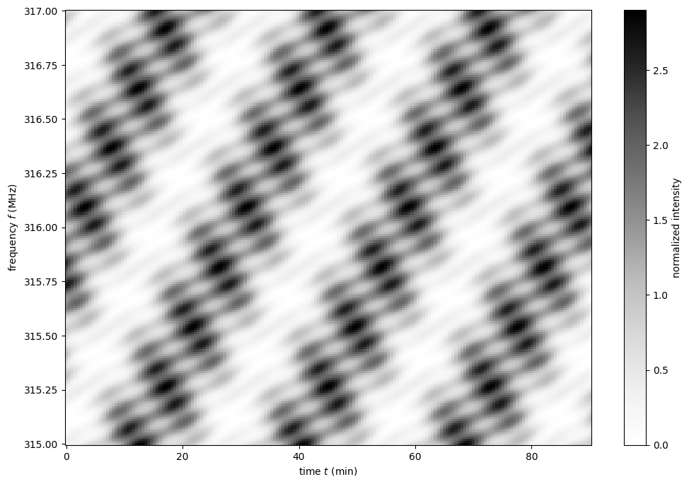
Making the dynamic spectrum
Define the observing frequencies and times. Make sure they will be broadcast against one another correctly.
t = np.linspace(0, 90*u.min, 180)[:, np.newaxis]
f = np.linspace(315*u.MHz, 317*u.MHz, 200)
Find the geometric delays as a function of time from the tau and taudot
attributes of obs1. Add two extra dimensions to accommodate the time and
frequency dimensions.
tau0 = obs1.tau[:, np.newaxis, np.newaxis]
taudot = obs1.taudot[:, np.newaxis, np.newaxis]
tau_t = tau0 + taudot * t
Compute the dynamic wavefield and then the dynamic spectrum. Here, we use the
phasor() function from screens.fields,
which essentially computes
np.exp(1j * (f * tau_t * u.cycle).to_value(u.rad)).
ph = phasor(f, tau_t)
brightness = obs1.brightness[:, np.newaxis, np.newaxis]
dynwave = ph * brightness

dynspec = np.abs(dynwave.sum(axis=0))**2
Plot the dynamic spectrum.
plt.figure(figsize=(12., 8.))

plt.imshow(dynspec.T,
           origin='lower', aspect='auto', interpolation='none',
           cmap='Greys', extent=axis_extent(t, f), vmin=0.)
plt.xlabel(rf"time $t$ ({t.unit.to_string('latex')})")
plt.ylabel(rf"frequency $f$ ({f.unit.to_string('latex')})")

cbar = plt.colorbar()
cbar.set_label('normalized intensity')
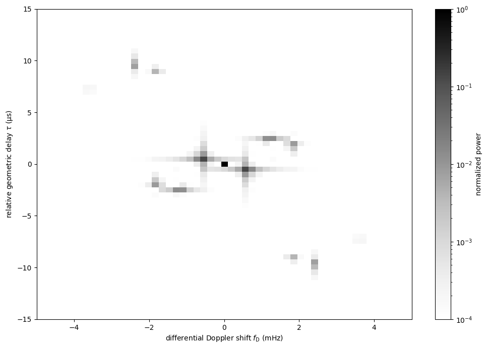
Making the secondary spectrum
Compute the conjugate spectrum, the conjugate variables, and then the secondary spectrum.
conjspec = np.fft.fft2(dynspec)
conjspec /= conjspec[0, 0]
conjspec = np.fft.fftshift(conjspec)

tau = np.fft.fftshift(np.fft.fftfreq(f.size, f[1]-f[0])).to(u.us)
fd = np.fft.fftshift(np.fft.fftfreq(t.size, t[1]-t[0])).to(u.mHz)

secspec = np.abs(conjspec)**2
Plot the secondary spectrum.
plt.figure(figsize=(12., 8.))

plt.imshow(secspec.T,
           origin='lower', aspect='auto', interpolation='none',
           cmap='Greys', extent=axis_extent(fd, tau),
           norm=LogNorm(vmin=1.e-4, vmax=1.))
plt.xlim(-5., 5.)
plt.ylim(-15., 15.)
plt.xlabel(r"differential Doppler shift $f_\mathrm{{D}}$ "
           rf"({fd.unit.to_string('latex')})")
plt.ylabel(r"relative geometric delay $\tau$ "
           rf"({tau.unit.to_string('latex')})")

cbar = plt.colorbar()
cbar.set_label('normalized power')

plt.show()
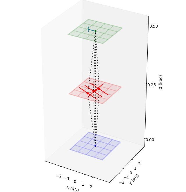
Visualize the system
Here is a bit of code that generates a 3D sketch of the system.
def unit_vector(c):
    return c.represent_as(UnitSphericalRepresentation).to_cartesian()

ZHAT = CartesianRepresentation(0., 0., 1., unit=u.one)

def plot_screen(ax, s, d, color='black', **kwargs):
    d = d.to_value(u.kpc)
    x = np.array(ax.get_xlim3d())
    y = np.array(ax.get_ylim3d())[:, np.newaxis]
    ax.plot_surface([[-2.1, 2.1]]*2, [[-2.1]*2, [2.1]*2], d*np.ones((2, 2)),
                    alpha=0.1, color=color)
    x = ax.get_xticks()
    y = ax.get_yticks()[:, np.newaxis]
    ax.plot_wireframe(x, y, np.broadcast_to(d, (x+y).shape),
                    alpha=0.2, color=color)
    spos = s.normal * s.p if isinstance(s, Screen1D) else s.pos
    ax.scatter(spos.x.to_value(u.AU), spos.y.to_value(u.AU), d,
               c=color, marker='+')
    if spos.shape:
        for pos in spos:
            zo = np.arange(2)
            ax.plot(pos.x.to_value(u.AU)*zo, pos.y.to_value(u.AU)*zo,
                    np.ones(2) * d, c=color, linestyle=':')
            upos = pos + (ZHAT.cross(unit_vector(pos)) * ([-1.5, 1.5] * u.AU))
            ax.plot(upos.x.to_value(u.AU), upos.y.to_value(u.AU),
                    np.ones(2) * d, c=color, linestyle='-')
    elif s.vel.norm() != 0:
        dp = s.vel * 5 * u.day
        ax.quiver(spos.x.to_value(u.AU), spos.y.to_value(u.AU), d,
                dp.x.to_value(u.AU), dp.y.to_value(u.AU), np.zeros(1),
                arrow_length_ratio=0.05)
plt.figure(figsize=(8., 12.))
ax = plt.subplot(111, projection='3d')
ax.set_box_aspect((1, 1, 2))
# ax.set_axis_off()
ax.grid(False)
ax.set_xlim3d(-4, 4)
ax.set_ylim3d(-4, 4)
ax.set_xticks([-2, -1, 0, 1., 2])
ax.set_yticks([-2, -1, 0, 1., 2])
ax.set_zticks([0, d_s.value, d_p.value])
ax.set_xlabel('x (AU)')
ax.set_ylabel('y (AU)')
ax.set_zlabel('z (kpc)', labelpad=12)
plot_screen(ax, telescope, 0*u.kpc, color='blue')
plot_screen(ax, scr1, d_s, color='red')
plot_screen(ax, pulsar, d_p, color='green')

path_shape = obs1.tau.shape
tpos = obs1.pos
scat1 = obs1.source.pos
ppos = obs1.source.source.pos
x = np.vstack(
    [np.broadcast_to(getattr(pos, 'x').to_value(u.AU), path_shape).ravel()
    for pos in (tpos, scat1, ppos)])
y = np.vstack(
    [np.broadcast_to(getattr(pos, 'y').to_value(u.AU), path_shape).ravel()
    for pos in (tpos, scat1, ppos)])
z = np.vstack(
    [np.broadcast_to(d, path_shape).ravel()
    for d in (0., d_s.value, d_p.value)])
for _x, _y, _z in zip(x.T, y.T, z.T):
    ax.plot(_x, _y, _z, color='black', linestyle=':')
    ax.scatter(_x[1], _y[1], _z[1], marker='o', color='red')