Simulating a multiple-screen system
This tutorial describes how to generate synthetic data corresponding to a
single-dish observation of a pulsar whose radiation is scattered by multiple
one-dimensional screens using the screens.screen module. It also
explains how to set up Screen1D objects from
patterns seen in a secondary spectrum, such that the synthetic data roughly
match the observations.
For background on the expected paths, see Scattering by multiple linear screens, and to visualize how the resulting wavefield depends on the properties of the screen, try examples/two_screen_interaction.py.
For the basics of how to use the Screen1D class and
the observe() method, please refer to the
preceding tutorial.
The numerical values in the example explored in this tutorial correspond to a model for the scattering of pulsar PSR B0834+06 from Hengrui Zhu et al. (2023), which is based on that of Liu et al. (2016).
The combined codeblocks in this tutorial can be downloaded as a Python script and as a Jupyter notebook:
- Python script:
- Jupyter notebook:
Preliminaries
Imports.
import numpy as np
import matplotlib.pyplot as plt
from matplotlib.colors import LogNorm

from astropy import units as u
from astropy import constants as const
from astropy.time import Time
from astropy.coordinates import (
    SkyCoord, SkyOffsetFrame, EarthLocation, CartesianRepresentation,
    CylindricalRepresentation, UnitSphericalRepresentation
)

from screens.screen import Source, Screen1D, Telescope
from screens.fields import phasor
# A handy function to help create an extent for matplotlib.pyplot.imshow
from screens.visualization import axis_extent
Define a matrix to transform between coordinate systems. This is needed because
Astropy’s SkyOffsetFrame yields frames where
the line of sight is along the x-axis, while the screens.screen
module assumes the line of sight is along the z-axis.
xyz2yzx = np.array([
    [0, 1, 0],
    [0, 0, 1],
    [1, 0, 0],
])
The pulsar
Set the pulsar’s distance, sky coordinates, and proper motion. Then create a
SkyOffsetFrame centered on the pulsar.
d_p = 0.620 * u.kpc

psr_coord = SkyCoord('08h37m5.644606s +06d10m15.4047s',
                     distance=d_p,
                     pm_ra_cosdec=2.16 * u.mas / u.yr,
                     pm_dec=51.64 * u.mas / u.yr)

psr_frame = SkyOffsetFrame(origin=psr_coord)
Get the pulsar’s velocity in the correct format.
vel_psr = (psr_coord
           .transform_to(psr_frame)
           .velocity
           .to_cartesian()
           .transform(xyz2yzx))
Create the Source object for the pulsar.
pulsar = Source(vel=vel_psr)
The telescope
Set the location of the telescope and the time of the observation. Use these
together with the get_gcrs() method
to get the telescope’s velocity.
tel_loc = EarthLocation('66°45′10″W', '18°20′48″N')

t_obs = Time(53712.29719907, format='mjd', scale='tai')

vel_tel = (tel_loc
           .get_gcrs(t_obs)
           .transform_to(psr_frame)
           .velocity
           .to_cartesian()
           .transform(xyz2yzx))
Create the Telescope object.
telescope = Telescope(vel=vel_tel)
The main screen
The screen properties
Set the distance of the screen from Earth \(d_\mathrm{s}\), the screen angle \(\xi\) (defined as the position angle of the line of lensed images, measured eastward from the celestial north), and the screen’s velocity along the line of lensed images \(v_\mathrm{lens,\parallel}\) (i.e., the component of the lens velocity in the direction defined by the angle \(\xi\)).
d_s1 = 0.389 * u.kpc
xi1 = 154.8 * u.deg
v_lens1 = 23.1 * u.km / u.s
The positions of main screen’s images
For screen 1 (the screen responsible for the main parabola in the secondary spectrum), we want to derive the positions of the images on the screen from the \(f_\mathrm{D}\) coordinates of the apices of the inverted arclets (measured in the secondary spectrum of the observation).
fd1 = [
    -15.93, -15.05, -14.47, -13.59, -13.00, -12.41, -11.83,  -9.78,
     -8.31,  -5.38,  -3.62,  -2.15,  -1.27,  -0.10,   1.08,   1.96,
      4.59,   5.47,   7.53,   9.29,  10.46,  15.15,
] * u.mHz
These could be converted to \(\theta\) angles using the main parabola’s curvature parameter \(\eta\), but since we have already set the screen’s distance and velocity, it’s better to do the conversion self-consistently using the screen’s effective velocity \(v_\mathrm{eff,\parallel}\), following
where \(\lambda\) is the observing wavelength.
First, get the component of the pulsar’s and the telescope’s (i.e., Earth’s) sky-plane velocity in the direction of the line of lensed images (see the tutorial on generating scintillation velocities for further explanation).
lens1_frame = SkyOffsetFrame(origin=psr_coord, rotation=xi1)

v_psr1 = psr_coord.transform_to(lens1_frame).velocity.d_z

v_tel1 = (tel_loc
          .get_gcrs(t_obs)
          .transform_to(lens1_frame)
          .velocity
          .d_z)
Then, compute effective velocity associated with the main screen.
s1 = 1. - d_s1 / d_p
v_eff1 = 1. / s1 * v_lens1 - (1. - s1) / s1 * v_psr1 - v_tel1
Finally, convert the listed \(f_\mathrm{D}\) coordinates to angles \(\theta\), and subsequently to positions on the screen (i.e., coordinates along the line of lensed images).
f_obs = 318.5 * u.MHz
lambda_obs = const.c / f_obs

theta1 = (lambda_obs * fd1 / v_eff1
         ).to(u.mas, equivalencies=u.dimensionless_angles())

pos1 = (theta1 * d_s1).to(u.au, equivalencies=u.dimensionless_angles())
Note
As a sanity check, we can verify that the curvature \(\eta\) corresponds to the value measured from the secondary spectrum.
d_eff1 = (1. - s1) / s1 * d_p

eta1 = lambda_obs**2 * d_eff1 / (2. * const.c * v_eff1**2)

eta1.to(u.s**3)
The magnifications of main screen’s images
The magnifications of the images on the main screen will be derived from the normalized brightness of the points along the main parabola with the \(f_\mathrm{D}\) coordinates listed above. We set random angles for the unknown intrinsic phase due to the lens.
brightness1 = [
      1.20,  1.66,  1.60,  1.45,  1.37,  0.99,  1.22,  8.99,
      8.51,  6.48, 22.04, 26.32, 28.05, 27.78, 22.64, 21.20,
     40.38, 18.76, 10.80,  6.31,  5.02,  0.21,
] * u.dimensionless_unscaled

rng = np.random.default_rng(seed=12345)
phase1 = rng.random(len(brightness1)) * 2.*np.pi

magnification1 = brightness1 / brightness1.max() * np.exp(1j*phase1)
Constructing the main screen
Create the Screen1D object for the main screen.
normal1 = CylindricalRepresentation(1., 90.*u.deg - xi1, 0.).to_cartesian()

screen1 = Screen1D(normal=normal1,
                   p=pos1,
                   v=v_lens1,
                   magnification=magnification1)
The second screen
Set the second screen’s properties.
d_s2 = 0.415 * u.kpc
xi2 =  46.1 * u.deg
v_lens2 = -3.3 * u.km / u.s
For the second screen, we manually set the position and magnification of the single image. In principle, these can be calculated from the coordinates and brightness of the millisecond feature in the secondary spectrum.
pos2 = [9.1652957] * u.au
magnification2 = 0.1
Create the Screen1D object for the second screen.
normal2 = CylindricalRepresentation(1., 90.*u.deg - xi2, 0.).to_cartesian()

screen2 = Screen1D(normal=normal2,
                   p=pos2,
                   v=v_lens2,
                   magnification=magnification2)
Generating observations
Use the observe() method to generate two sets
of optical paths: one for radiation scattered only by the main screen
(resulting in the main parabola) and one for radiation scattered by both
screens (yielding the millisecond feature).
obs1 = telescope.observe(
    source=screen1.observe(source=pulsar, distance=d_p-d_s1),
    distance=d_s1)

obs2 = telescope.observe(
    source=screen1.observe(
        source=screen2.observe(source=pulsar, distance=d_p-d_s2),
        distance=d_s2-d_s1),
    distance=d_s1)
The Screen1D class assumes that the linear features
that cause the images on the lens continue indefinitely. The lens that causes
the millisecond feature, however, is found to be limited in extent, not
producing any scatterings beyond a certain point on the sky. To model this, we
have to use a little hack: we can select optical paths in obs2 based on
their positions at the main screen. For these positions to be available, they
first need to be computed. This is triggered by the first line, which computes
the geometric delays of the optical paths, for which the positions of the
scattering points on both screens need to be calculated.
obs2.tau
bool_on_lens2 = obs2.source.pos.x.ravel() < 7. * u.au
Using the tau, taudot, and brightness attributes of obs1 and
obs2, we can find the geometric delays of the optical paths (at the
reference time), their time derivatives, and their complex magnifications. We
combine the two sets of optical paths into a single list, using only the ones
from obs2 that were selected above using bool_on_lens2.
tau0 = np.hstack([obs1.tau.ravel(),
                  obs2.tau.ravel()[bool_on_lens2]])
taudot = np.hstack([obs1.taudot.ravel(),
                    obs2.taudot.ravel()[bool_on_lens2]])
brightness = np.hstack([obs1.brightness.ravel(),
                        obs2.brightness.ravel()[bool_on_lens2]])
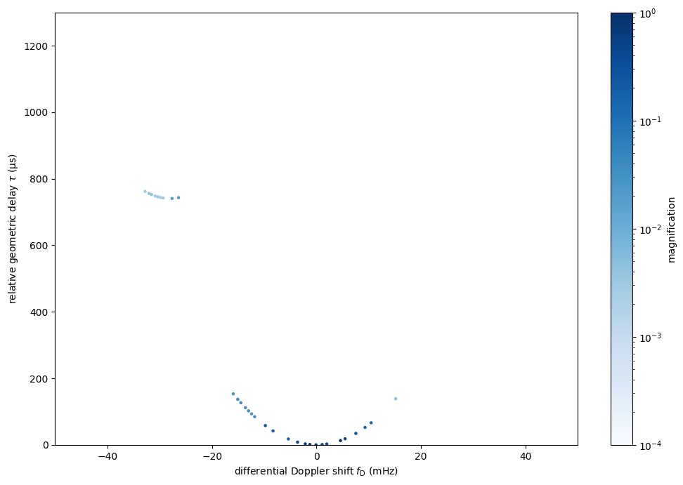
Plot the optical paths in conjugate variable space (the Doppler shift can be expressed as \(f_\mathrm{D} = f_\mathrm{obs} \dot{\tau}\), where \(f_\mathrm{obs}\) is the observing frequency). This figure should correspond to the norm of the conjugate wavefield, showing the arclet apices with their associated magnifications.
fd_all = f_obs * taudot

plt.figure(figsize=(12., 8.))

plt.scatter(fd_all.to(u.mHz), tau0.to(u.us),
            c=np.abs(brightness).value, s=5, cmap='Blues',
            norm=LogNorm(vmin=1.e-4, vmax=1.))

plt.xlim(-50., 50.)
plt.ylim(0., 1300.)
plt.xlabel(r"differential Doppler shift $f_\mathrm{{D}}$ (mHz)")
plt.ylabel(r"relative geometric delay $\tau$ ($\mathrm{\mu s}$)")

cbar = plt.colorbar()
cbar.set_label('magnification')

plt.show()
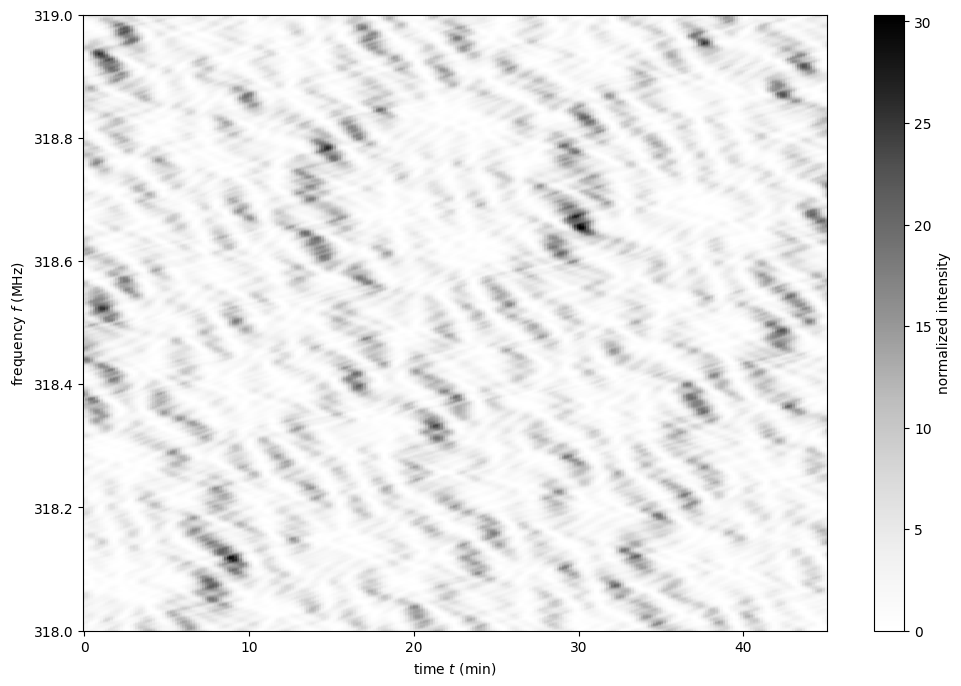
Making the dynamic spectrum
Define the observing frequencies and times. Make one a column vector and the other a row vector, so they will be broadcast against one another correctly.
t = np.linspace(0, 45*u.min, 300)[:, np.newaxis]
f = np.linspace(318.*u.MHz, 319.*u.MHz, 3000)
Compute the geometric delays as a function of time, the associated geometric phases, then the dynamic wavefield, and finally the dynamic spectrum.
tau_t = (tau0[:, np.newaxis, np.newaxis]
        + taudot[:, np.newaxis, np.newaxis] * t)

ph = phasor(f, tau_t)

dynwave = ph * brightness[:, np.newaxis, np.newaxis]

dynspec = np.abs(dynwave.sum(0))**2
Plot the dynamic spectrum.
plt.figure(figsize=(12., 8.))

plt.imshow(dynspec.T,
           origin='lower', aspect='auto', interpolation='none',
           cmap='Greys', extent=axis_extent(t, f), vmin=0.)
plt.xlabel(rf"time $t$ ({t.unit.to_string('latex')})")
plt.ylabel(rf"frequency $f$ ({f.unit.to_string('latex')})")

cbar = plt.colorbar()
cbar.set_label('normalized intensity')
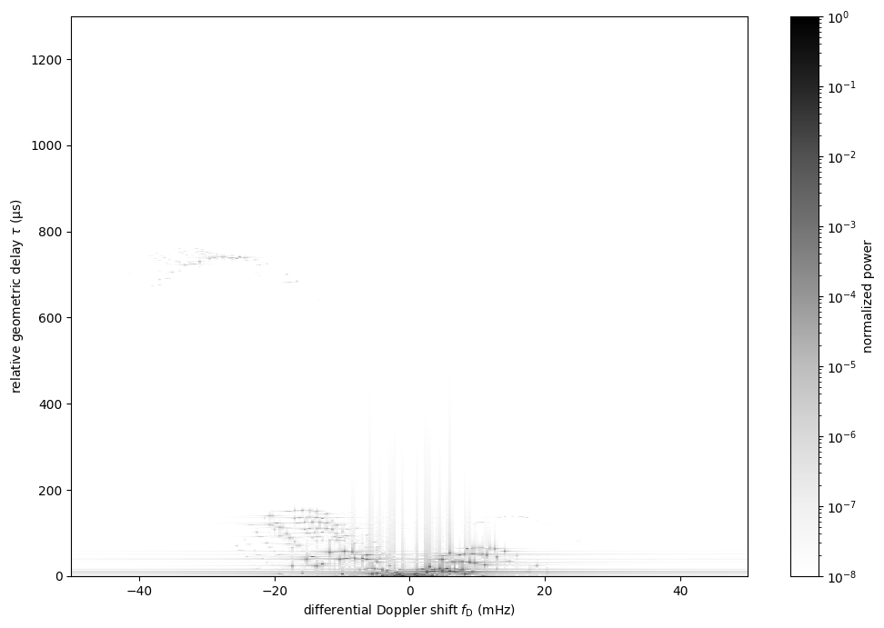
Making the secondary spectrum
Compute the conjugate spectrum, the conjugate variables, and then the secondary spectrum.
conjspec = np.fft.fft2(dynspec)
conjspec /= conjspec[0, 0]
conjspec = np.fft.fftshift(conjspec)

tau = np.fft.fftshift(np.fft.fftfreq(f.size, f[1]-f[0])).to(u.us)
fd = np.fft.fftshift(np.fft.fftfreq(t.size, t[1]-t[0])).to(u.mHz)

secspec = np.abs(conjspec)**2
Plot the secondary spectrum.
plt.figure(figsize=(12., 8.))

plt.imshow(secspec.T.value,
           origin='lower', aspect='auto', interpolation='none',
           cmap='Greys', extent=axis_extent(fd, tau),
           norm=LogNorm(vmin=1.e-8, vmax=1.))

plt.xlim(-50., 50.)
plt.ylim(0., 1300.)
plt.xlabel(r"differential Doppler shift $f_\mathrm{{D}}$ "
           rf"({fd.unit.to_string('latex')})")
plt.ylabel(r"relative geometric delay $\tau$ "
           rf"({tau.unit.to_string('latex')})")

cbar = plt.colorbar()
cbar.set_label('normalized power')

plt.show()
Overplot the arclet apices.
plt.figure(figsize=(12., 8.))

plt.imshow(secspec.T.value,
           origin='lower', aspect='auto', interpolation='none',
           cmap='Greys', extent=axis_extent(fd, tau),
           norm=LogNorm(vmin=1.e-8, vmax=1.))

plt.xlim(-50., 50.)
plt.ylim(0., 1300.)
plt.xlabel(r"differential Doppler shift $f_\mathrm{{D}}$ "
           rf"({fd.unit.to_string('latex')})")
plt.ylabel(r"relative geometric delay $\tau$ "
           rf"({tau.unit.to_string('latex')})")

cbar = plt.colorbar()
cbar.set_label('normalized power')

plt.scatter(fd_all.to(u.mHz), tau0.to(u.us),
            c=np.abs(brightness).value, s=5, cmap='Blues',
            norm=LogNorm(vmin=1.e-4, vmax=1.))

cbar = plt.colorbar()
cbar.set_label('magnification')

plt.show()
