Simulating VLBI Data
This tutorial describes how to generate synthetic data corresponding to a VLBI observation of a pulsar whose radiation is scattered by a single one-dimensional screen using the screens.screen module.
This simulation is based around the results of Hengrui Zhu’s work on PSR B0834+06.
For the basics of how to use the Screen1D
class, see Using the Screen1D class.
The code used in this example can be downloaded from:
- Python script:
- Jupyter notebook:
Import
Import some useful functions for simulating screens.
import numpy as np

import matplotlib.pyplot as plt
from matplotlib.colors import LogNorm, SymLogNorm

import astropy.constants as const
import astropy.units as u
from astropy.coordinates import (
    CartesianRepresentation,
    CylindricalRepresentation,
    EarthLocation,
    SkyCoord,
    SkyOffsetFrame,
)
from astropy.time import Time

from screens.fields import phasor
from screens.screen import Screen1D, Source, Telescope
from screens.visualization import axis_extent
# Set random seed, to allow checking result doesn't change with edits.
np.random.seed(12345)
Simulation Function
For convenience we have collected the simulation code into a single function.
def simulate(pulsar, d_scr, v_scr, pa_scr, n_image, time, freq, dishes):
    """
    Simulation Code

    Parameters
    ----------
    pulsar : ~astropy.coordiantes.SkyCoord
        Must have RA, Dec, distance, and proper motion.
    d_scr : ~astropy.units.Quantity
        Distance to screen from Earth.
    v_scr : ~astropy.units.Quantity
        Velocity of the screen along the line of images
    pa_scr : ~astropy.units.Quantity
        Orientation of line of images defined E of N
    n_image : int
        The number of images to simulate.
    time : ~astropy.time.Time
        Times of the observation, with shape (n_time, 1)
    freq : ~astropy.units.Quantity
        Array of channel frequencies, with shape (n_freq,)
    dishes : dict of ~astropy.coordinates.EarthLocation
        Keyed by the dish identifiers.
    """

    # Create pulsar frame and initialize the source.
    psr_frame = SkyOffsetFrame(origin=pulsar)
    d_psr = pulsar.distance
    # Velocity in RA, Dec, radial order.
    v_psr = pulsar.transform_to(psr_frame).cartesian.differentials["s"]
    source = Source(vel=CartesianRepresentation(v_psr.d_y, v_psr.d_z, v_psr.d_z))

    # Convert time and freq for use in screens
    t = (time-time[0]).to(u.min)[:, np.newaxis]
    f = np.copy(freq)

    # Calculate useful derived quanities
    d_eff = d_psr * d_scr / (d_psr - d_scr)

    fd = np.fft.fftshift(np.fft.fftfreq(t.shape[0], d=t[1]-t[0]).to(u.mHz))
    tau = np.fft.fftshift(np.fft.fftfreq(f.shape[0], d=f[1]-f[0]).to(u.us))

    # Determine furthest image observable in data (tau limit)
    theta_max = np.sqrt(0.8 * 2 * tau.max() * const.c / d_eff)

    # Create Screen
    p_scr = np.random.uniform(-1, 1, n_image) << u.one
    p_scr[0] = 0
    m_scr = np.exp(-0.5*(p_scr/10)**2) * np.exp(
        1j * np.random.uniform(-np.pi, np.pi, n_image)
    )
    m_scr /= np.sqrt(np.sum(np.abs(m_scr)**2))
    p_scr *= theta_max * d_scr

    n_scr = CylindricalRepresentation(
        1.0, 90 * u.deg - pa_scr, 0.0).to_cartesian()

    screen = Screen1D(normal=n_scr, p=p_scr, v=v_scr, magnification=m_scr)

    # Observe pulsar with screen
    scr_psr = screen.observe(source=source, distance=d_psr - d_scr)

    # Results to store (keyed by name)
    uvw = {}
    wavefields = {}
    # Determine Earth core position in pulsar frame (relative to SSB)
    center_of_earth = EarthLocation(0, 0, 0, unit=u.m).get_itrs(time.mean())
    center_of_earth = center_of_earth.transform_to(psr_frame).cartesian
    # Loop over all dishes
    for name, loc in dishes.items():
        # Get dish location to pulsar frame at the middle of the observation
        # (here, gcrs instead of itrs to also get velocity).
        dish_pos = loc.get_gcrs(time.mean()).transform_to(psr_frame).cartesian

        # Dish position relative to earth center in UVW, and velocity.
        dish_uvw = dish_pos.without_differentials() - center_of_earth
        dish_vel = dish_pos.differentials["s"].to_cartesian()

        uvw[name] = dish_uvw

        # Create telescope and observe the screen with it.
        telescope = Telescope(
            pos=CartesianRepresentation(dish_uvw.y, dish_uvw.z, dish_uvw.x),
            vel=CartesianRepresentation(dish_vel.y, dish_vel.z, dish_vel.x),
        )
        obs = telescope.observe(source=scr_psr, distance=d_scr)

        # Create wavefield.
        brightness = obs.brightness[:, np.newaxis, np.newaxis]
        tau0 = obs.tau[:, np.newaxis, np.newaxis]
        taudot = obs.taudot[:, np.newaxis, np.newaxis]
        tau_t = tau0 + taudot * t
        ph = phasor(freq, tau_t, linear_axis=-1)
        wavefields[name] = np.sum(ph * brightness.to_value(u.one), axis=0).T

    # Create visibilities
    spectra = {}
    for i, name1 in enumerate(dishes):
        for name2 in list(dishes)[i:]:
            spectra[name1, name2] = wavefields[name1] * wavefields[name2].conj()

    return spectra, uvw, wavefields
Parameters
Define simulation parameters.
Pulsar
In this simulation we use the parameters from pulsar B0834+06.
pulsar = SkyCoord(ra="8h37m05.6485930s", dec="6d10m16.06361s",
                  distance=0.620 * u.kpc,
                  pm_ra_cosdec=2.16*u.mas/u.yr, pm_dec=51.64*u.mas/u.yr)
Screen
For the interstellar screen, we use 100 images to produce nice dynamic and conjugate spectra. The other screen parameters are based on Hengrui Zhu’s work.
screen_pars = dict(
     n_image=100,
     d_scr=0.389 * u.kpc,
     pa_scr=154.8*u.deg,
     v_scr=23.1*u.km/u.s,
)
Observation
For this simulation, we simulate 1 hour of data on MJD 53675 for a 1 MHz band from 318 MHz to 319 MHz on the Green Bank and dearly missed Arecibo telescopes.
# Locations from PINT: src/pint/observatory/observatories.py
dishes = {
    "AO": EarthLocation(2390487.080, -5564731.357, 1994720.633, unit="m"),
    "GB" : EarthLocation(882589.289, -4924872.368, 3943729.418, unit="m"),
}
time = Time(53675, np.linspace(0, 1, 512)/24, format="mjd")
freq = np.linspace(318,319,1024) << u.MHz
obs_pars = dict(time=time, freq=freq, dishes=dishes)
Simulation
Now construct simulated dynamic and visibility spectra using the above parameters. The spectra are keyed by tuples of the names. For diagnostic purposes, also returned are the UVW for each station, as well as the underlying wavefields.
spectra, uvw, wavefields = simulate(pulsar, **screen_pars, **obs_pars)
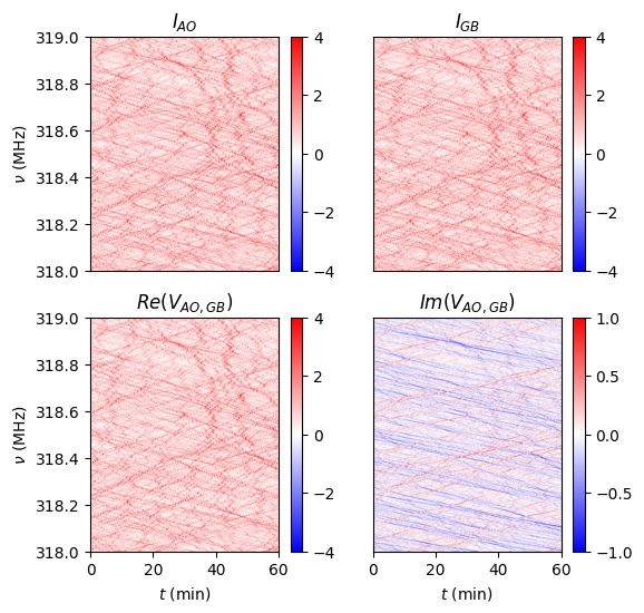
Looking at the the resulting spectra, we see that the visiblity is predominantly positive, real, and very similar to the dynamic spectra. The imaginary part is much smaller and contains the expected cross hatch pattern of positive and negative features along opposite diagonals.
names = list(dishes)
imshow_kwargs = dict(origin='lower', aspect='auto', cmap='bwr',
                     extent=axis_extent((time-time[0]).to(u.min), freq))
grid = plt.GridSpec(nrows=2, ncols=2)
plt.figure(figsize=(6, 6))
plt.subplot(grid[0, 0])
plt.imshow(spectra[names[0], names[0]].real, vmin=-4, vmax=4, **imshow_kwargs)
plt.ylabel(r'$\nu~\left(\rm{MHz}\right)$')
plt.xticks([])
plt.title(rf'$I_{{{names[0]}}}$')
plt.colorbar()
plt.subplot(grid[0, 1])
plt.imshow(spectra[names[1], names[1]].real, vmin=-4, vmax=4, **imshow_kwargs)
plt.yticks([])
plt.xticks([])
plt.title(rf'$I_{{{names[1]}}}$')
plt.colorbar()
plt.subplot(grid[1, 0])
plt.imshow(spectra[names[0], names[1]].real, vmin=-4, vmax=4, **imshow_kwargs)
plt.ylabel(r'$\nu~\left(\rm{MHz}\right)$')
plt.xlabel(r'$t~\left(\rm{min}\right)$')
plt.title(rf'$Re\left(V_{{{names[0]},{names[1]}}}\right)$')
plt.colorbar()
plt.subplot(grid[1, 1])
plt.imshow(spectra[names[0], names[1]].imag, vmin=-1, vmax=1, **imshow_kwargs)
plt.yticks([])
plt.xlabel(r'$t~\left(\rm{min}\right)$')
plt.title(rf'$Im\left(V_{{{names[0]},{names[1]}}}\right)$')
plt.colorbar()
<matplotlib.colorbar.Colorbar at 0x77fc0ed334d0>