Generating synthetic scintillation velocities
This tutorial describes how to generate synthetic scintillation velocities for a pulsar in a circular orbit and a single one-dimensional screen, both with known parameters.
For a derivation of the equations seen here, refer to the scintillation velocities background. Further explanations can be found in Marten’s scintillometry page and Daniel Baker’s “Orbital Parameters and Distances” document. As in that document, the practical example here uses the parameter values for the pulsar PSR J0437–4715 as derived by Reardon et al. (2020).
The combined codeblocks in this tutorial can be downloaded as a Python script and as a Jupyter notebook:
- Python script:
- Jupyter notebook:
Preliminaries
Imports.
import numpy as np
import matplotlib.pyplot as plt

from astropy import units as u
from astropy import constants as const

from astropy.time import Time
from astropy.coordinates import SkyCoord, SkyOffsetFrame, EarthLocation

from astropy.visualization import quantity_support, time_support
Set up support for plotting Astropy’s
Quantity and Time
objects, and make sure that the output of plotting commands is displayed inline
(i.e., directly below the code cell that produced it).
quantity_support()
time_support(format='iso')

%matplotlib inline
Initializing parameters
Set the parameters of the pulsar system:
Parameter |
Symbol |
Remarks |
|---|---|---|
Coordinates of the pulsar system |
||
right ascension |
\(\alpha_\mathrm{p}\) |
|
declination |
\(\delta_\mathrm{p}\) |
|
proper motion in right ascension |
\(\mu_\mathrm{p,sys,\alpha\ast}\) |
including the \(\cos(\delta_\mathrm{p})\) term |
proper motion in declination |
\(\mu_\mathrm{p,sys,\delta}\) |
|
Orbital elements of the pulsar binary |
||
binary period |
\(P_\mathrm{orb,p}\) |
|
projected semi-major axis |
\(a_\mathrm{p} \sin( i_\mathrm{p} )\) |
|
orbital inclination |
\(i_\mathrm{p}\) |
\(0^\circ \leq i_\mathrm{p} < 180^\circ\), with \(i_\mathrm{p} = 90^\circ\) for an edge-on orbit; for \(i_\mathrm{p} < 90^\circ\), the binary rotates counterclockwise on the sky (from north through east), for \(i_\mathrm{p} \geq 90^\circ\) it rotates clockwise |
longitude of ascending node |
\(\Omega_\mathrm{p}\) |
measured from the celestial north through east; \(0^\circ \leq \Omega_\mathrm{p} < 360^\circ\) |
time of ascending node |
\(t_\mathrm{asc,p}\) |
|
Further parameters |
||
distance to the pulsar system |
\(d_\mathrm{p}\) |
|
distance to the screen |
\(d_\mathrm{s}\) |
from Earth |
position angle of the lensed images |
\(\xi\) |
measured from the celestial north, through east, to the line of images formed by the lens; \(0^\circ \leq \xi < 180^\circ\) |
velocity of the lens |
\(v_\mathrm{lens,\parallel}\) |
component along the screen direction |
p_orb_p = 5.7410459 * u.day
asini_p = 3.3667144 * const.c * u.s
i_p = 137.56 * u.deg
omega_p = 207. * u.deg
t_asc_p = Time(54501.4671, format='mjd', scale='tdb')

d_p = 156.79 * u.pc
d_s = 90.6 * u.pc
xi = 134.6 * u.deg
v_lens = -31.9 * u.km / u.s
The coordinates should be placed directly in a
SkyCoord object, that includes the pulsar
system’s position on the sky, its distance, and its proper motion.
psr_coord = SkyCoord('04h37m15.99744s -47d15m09.7170s',
                     distance=d_p,
                     pm_ra_cosdec=121.4385 * u.mas / u.yr,
                     pm_dec=-71.4754 * u.mas / u.yr)
Calculate some derived quantities:
Parameter |
Equation |
|---|---|
pulsar’s radial-velocity amplitude |
\[K_\mathrm{p} = \frac{ 2 \pi a_\mathrm{p} \sin( i_\mathrm{p} ) }
{ P_\mathrm{orb,p} }\]
|
fractional distance to the screen (from the pulsar) |
\[s = 1 - \frac{ d_\mathrm{s} }{ d_\mathrm{p} }\]
|
effective distance |
\[d_\mathrm{eff} = \frac{ 1 - s }{ s } d_\mathrm{p}\]
|
angle from the pulsar’s ascending node to the line of lensed images |
\[\Delta\Omega_\mathrm{p} = \xi - \Omega_\mathrm{p}\]
|
k_p = 2.*np.pi * asini_p / p_orb_p

s = 1 - d_s / d_p
d_eff = d_p * d_s / (d_p - d_s)

delta_omega_p = xi - omega_p
Define a grid of observing times \(t\) for which you want to calculate
velocities using a Time object.
t_mjd = np.arange(55000., 55700., 0.25)
t = Time(t_mjd, format='mjd', scale='utc')
The lens frame
Make a SkyOffsetFrame centered on the pulsar
system, rotated to the one-dimensional lens.
lens_frame = SkyOffsetFrame(origin=psr_coord, rotation=xi)
On its own, SkyOffsetFrame(origin=psr_coord) creates a spherical frame with
its primary direction pointing along the line of sight, latitude in the
direction of Dec, and longitude in the direction of RA. By passing the argument
rotation=xi, the longitude and latitude dimensions rotate so longitude
is perpedicular to the lens and latitude parallel to the lens. When converting
positions or velocities in this frame to cartesian representation, the x-axis
will point along the line of sight, the y-axis perpendicular to the screen, and
the z-axis parallel to the screen (in the direction of its motion). Hence, we
need to compute the cartesian z-component of velocities in lens_frame.
Calculating effective velocities
There are several components of the effective velocity that can be computed separately:
Velocity component |
Symbol |
|---|---|
Earth’s velocity as a function of time |
\(v_{\oplus,\parallel}( t )\) |
pulsar’s orbital velocity as a function of time |
\(v_\mathrm{p,orb,\parallel}( t )\) |
pulsar systemic velocity (corresponding to the proper motion) |
\(v_\mathrm{p,sys,\parallel}\) |
velocity of the lens (known in this example) |
\(v_\mathrm{lens,\parallel}\) |
All these refer to the component of the velocity along the line of images formed by the lens.
Earth’s velocity
To obtain Earth’s velocity in the lens frame, first generate a location on
Earth’s surface using the EarthLocation class
(in this case the location of the Parkes radio telescope). This class has the
get_gcrs() method, which returns
positions (with respect to the centre of the Earth) as a function of time.
These are transformed into the lens frame using the
transform_to() method.
Velocities can then be extracted using the
velocity attribute, and
finally d_z isolates the
z-component of the velocity (in the direction of the screen).
earth_loc = EarthLocation('148°15′47″E', '32°59′52″S')

v_earth = earth_loc.get_gcrs(t).transform_to(lens_frame).velocity.d_z
Pulsar’s orbital velocity
Compute the pulsar’s orbital velocity projected onto the screen
Here, \(\phi_\mathrm{p}( t )\) is the phase of pulsar orbit as measured from its ascending node.
ph_p = ((t - t_asc_p) / p_orb_p).to(u.dimensionless_unscaled) * u.cycle

v_p_orb = (-k_p / np.sin(i_p)
            * (np.cos(delta_omega_p) * np.sin(ph_p)
             - np.sin(delta_omega_p) * np.cos(i_p) * np.cos(ph_p)))
Pulsar systemic velocity
The pulsar systemic velocity projected onto the screen is given by
This can be computed manually, but it can also be retrieved from the
SkyCoord of the pulsar system (which contains
the system’s proper motion) by transforming it to lens_frame.
v_p_sys = psr_coord.transform_to(lens_frame).velocity.d_z
Effective velocity
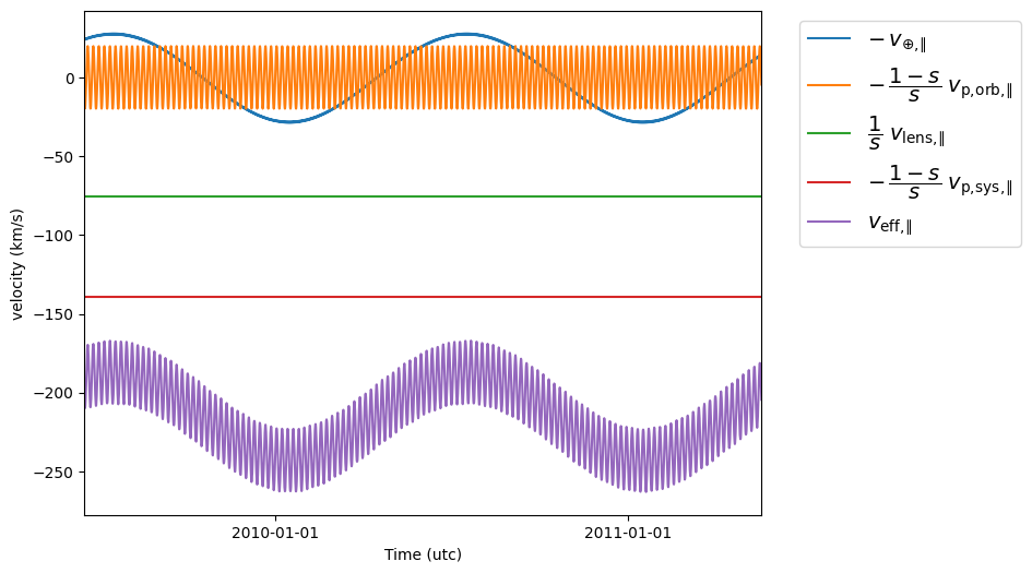
Combine the velocities of the pulsar, Earth, and the lens into the effective velocity
v_eff = 1. / s * v_lens - (1. - s) / s * (v_p_sys + v_p_orb) - v_earth
Have a look at the contribution of each of the terms to the effective velocity.
plt.figure(figsize=(8., 6.))

plt.plot(t, - v_earth)
plt.plot(t, - ((1. - s) / s) * v_p_orb)
plt.plot(t[::len(t)-1], 1. / s * v_lens * [1., 1.])
plt.plot(t[::len(t)-1], - ((1. - s) / s) * v_p_sys * [1., 1.])
plt.plot(t, v_eff)
plt.legend([r'$- \, v_{\oplus,\!\!\parallel}$',
            r'$- \, \dfrac{ 1 - s }{ s } \; v_\mathrm{p,\!orb,\!\!\parallel}$',
            r'$\dfrac{ 1 }{ s } \; v_\mathrm{lens,\!\!\parallel}$',
            r'$- \, \dfrac{ 1 - s }{ s } \; v_\mathrm{p,\!sys,\!\!\parallel}$',
            r'$v_\mathrm{eff,\!\!\parallel}$'],
           bbox_to_anchor=(1.04, 1.), loc='upper left', fontsize=14)
plt.xlim(t[0], t[-1])
plt.ylabel(r'velocity (km/s)')

plt.show()
Curvature and scaled effective velocity
The curvature \(\eta\) can be computed from the effective velocity according to
where \(\lambda\) is the observing wavelength and \(c\) is the speed of light.
lambda_obs = (1400. * u.MHz).to(u.m, equivalencies=u.spectral())

eta = lambda_obs**2 * d_eff / (2. * const.c * v_eff**2)
Have a look at the curvature at a function of time.
plt.figure(figsize=(10., 6.))

plt.plot(t, eta.to(u.s**3))
plt.xlim(t[0], t[-1])
plt.ylabel(r'curvature $\eta$ (s$^3$)')

plt.show()
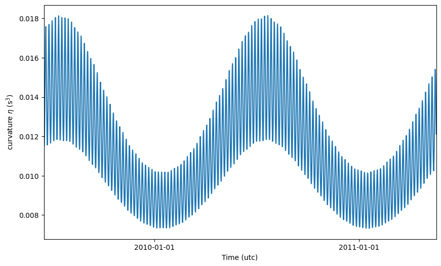
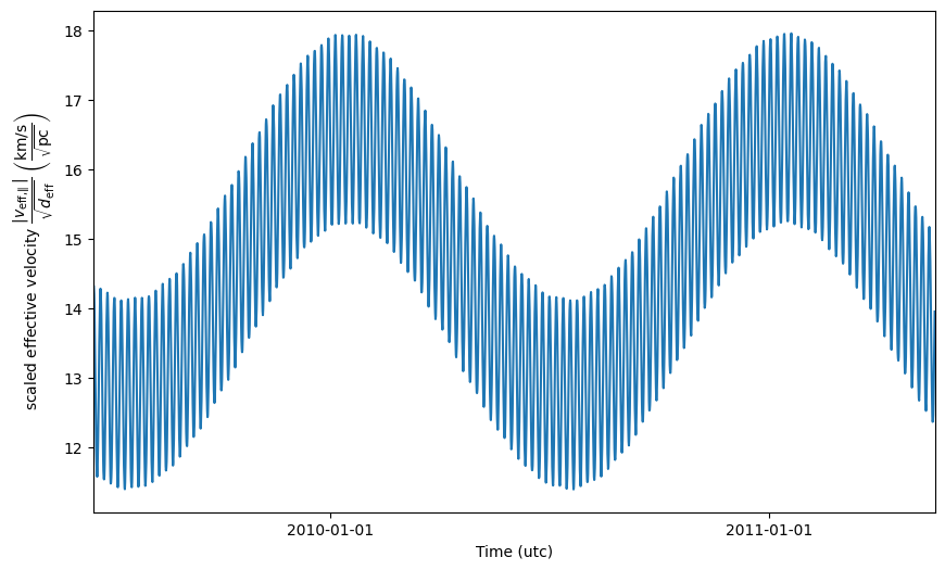
Since \(v_\mathrm{eff}\) can be arbitrarily close to zero (letting \(\eta\) blow up), curvature has a strongly non-uniform prior probability distribution (as can be seen from the modulation in amplitude in the figure above). For this reason, it is sometimes better to fit for the curvature of the secondary spectrum parabola in a space of “scaled effective velocity”
dveff = np.abs(v_eff) / np.sqrt(d_eff)
Plot this quantity as function of time.
plt.figure(figsize=(10., 6.))

plt.plot(t, dveff)
plt.xlim(t[0], t[-1])
dveff_lbl = (r'scaled effective velocity '
             r'$\dfrac{ | v_\mathrm{eff,\!\!\parallel} | }'
             r'{ \sqrt{ d_\mathrm{eff} } }$ '
             r'$\left( \dfrac{\mathrm{km/s}}{\sqrt{\mathrm{pc}}} \right)$')
plt.ylabel(dveff_lbl)

plt.show()
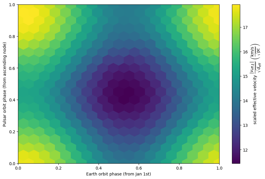
To visualize the modulation in scintillation velocity caused by both the pulsar’s orbital motion and that of the Earth, we can make a 2D phase fold of the data.
plt.figure(figsize=(11., 7.))

plt.hexbin(t.jyear % 1., ph_p.value % 1., C=dveff.value,
           reduce_C_function=np.median, gridsize=19)
plt.xlim(0., 1.)
plt.ylim(0., 1.)
plt.xlabel('Earth orbit phase (from Jan 1st)')
plt.ylabel('Pulsar orbit phase (from ascending node)')
cbar = plt.colorbar()
cbar.set_label(dveff_lbl)

plt.show()
Generate noisy synthetic observations
We now want to generate a set of noisy scaled effective velocities, to use in the next tutorial, in which we will fit a model to these fake observations.
To start, we create a set of irregularly spaced observation times.
np.random.seed(654321)
nt = 2645
dt_mean = 16.425 * u.yr / nt
dt = np.random.random(nt) * 2. * dt_mean
t = Time(52618., format='mjd') + dt.cumsum()
Next, the time-dependent parts of the above calculations need to be repeated for the new times.
v_earth = earth_loc.get_gcrs(t).transform_to(lens_frame).velocity.d_z

ph_p = ((t - t_asc_p) / p_orb_p).to(u.dimensionless_unscaled) * u.cycle

v_p_orb = (-k_p / np.sin(i_p)
            * (np.cos(delta_omega_p) * np.sin(ph_p)
            - np.sin(delta_omega_p) * np.cos(i_p) * np.cos(ph_p)))

v_eff = 1. / s * v_lens - (1. - s) / s * (v_p_orb + v_p_sys) - v_earth

dveff = np.abs(v_eff) / np.sqrt(d_eff)
Now we add some noise to the scaled effective velocities.
dveff_err = (np.random.random(nt) * 0.05 + 0.05) * np.mean(dveff)
dveff_obs = dveff + dveff_err * np.random.normal(size=nt)
Finally, we use NumPy’s savez() to save the data as a set of
(unitless) NumPy arrays.
np.savez('data/fake-data-J0437.npz',
         t_mjd=t.mjd,
         dveff_obs=dveff_obs.value,
         dveff_err=dveff_err.value)