Error analysis

This tutorial describes how to propagate (a) the statistical uncertainties on the parameters of a model that was fit to a time series of scintillation velocities to (b) uncertainties on the physical parameters that describe the pulsar system and the scattering screen. The model assumes a pulsar on a circular orbit whose radiation is scattered by a single one-dimensional screen. The tutorial builds upon a preceding tutorial that described in more detail how the physical parameters can be inferred from the model parameters. Like in the second part of that tutorial, this error-propagation tutorial assumes there are some constraints on the distance to the pulsar. The tutorial uses the fit results generated in the tutorial on fitting scintillation velocities. These fit results are available for download: fit-results-J0437.npz

We will do error propagation using two methods:

• Monte Carlo sampling, using Astropy’s uncertainty module.

• Linear error propagation, using the uncertainties package.

The analysis in this tutorial does not (yet) consider the prior probabilities on parameters such as the flat distribution in \(\cos(i_\mathrm{p})\) for the pulsar’s orbital inclination \(i_\mathrm{p}\).

For a derivation of the equations seen here, refer to the scintillation velocities background. Further explanations can be found in Marten’s scintillometry page and Daniel Baker’s “Orbital Parameters and Distances” document. As in that document, the practical example here uses the parameter values for the pulsar PSR J0437–4715 as derived by Reardon et al. (2020), except for the pulsar distance (we use an inflated uncertainty on the distance, so the example is more representative of typical pulsar distance estimates).

The combined codeblocks in this tutorial can be downloaded as a Python script and as a Jupyter notebook:

Python script:

error_analysis.py

Jupyter notebook:

error_analysis.ipynb

Preliminaries

Imports.

import numpy as np
import matplotlib.pyplot as plt

from matplotlib.patches import Ellipse

from astropy import units as u
from astropy import constants as const
from astropy import uncertainty as unc

from astropy.time import Time
from astropy.coordinates import SkyCoord

from uncertainties import ufloat, umath, correlated_values, covariance_matrix

from scipy import stats as st

import corner
from IPython.display import display, Math

from collections import namedtuple

Set a seed for the random number generator to make the results reproducable.

np.random.seed(654321)

Set some defaults for plotting functions, including the levels at which to draw confidence contours in 2D (see the note about sigmas in the documentation of the corner package)

contour2d_sigmas = np.array([1., 2.])
contour2d_levels = 1.0 - np.exp(-0.5 * contour2d_sigmas**2)

corner_kwargs = {
    'levels':       contour2d_levels,
    'hist_kwargs':  {'density': True},
    'label_kwargs': {'size': 12},
}

linear_style = {
    'linestyle': '-',
    'linewidth': 1.5,
    'color':     'C1',
}

figsize_inches = (9.5, 9.5)

Define a function to overplot the results of linear error propagation on an existing corner plot (Gaussian probability density curves in the panels along the diagonal, confidence ellipses in the off-diagonal panels).

def overplot_linear(fig, upars, mahalanobis_radii=contour2d_sigmas, **kwargs):

    # get optimal values, standard deviations and covariance matrix
    opt = [upar.n for upar in upars]
    std = [upar.s for upar in upars]
    cov = covariance_matrix(upars)

    npoints = 100

    ndim = len(upars)
    axes = np.array(fig.axes).reshape((ndim, ndim))

    # Gaussian probability density curves
    for i in range(ndim):
        ax = axes[i, i]
        xlims = ax.get_xlim()

        x = np.linspace(xlims[0], xlims[1], npoints)
        y = st.norm.pdf(x, opt[i], std[i])

        ax.plot(x, y, **kwargs)

    # confidence ellipses
    for yi in range(ndim):
        for xi in range(yi):
            ax = axes[yi, xi]

            # ellipse centre
            opt_xy = (opt[xi], opt[yi])

            # get covariances
            cov_xx = cov[xi][xi]
            cov_yy = cov[yi][yi]
            cov_xy = cov[xi][yi]

            # compute eigenvalues and ellipse orientation
            lambda_a = ((cov_xx + cov_yy) / 2.
                        + np.sqrt((cov_xx - cov_yy)**2 / 4. + cov_xy**2))
            lambda_b = ((cov_xx + cov_yy) / 2.
                        - np.sqrt((cov_xx - cov_yy)**2 / 4. + cov_xy**2))
            theta = np.arctan2(2. * cov_xy, cov_xx - cov_yy) / 2.

            for r in mahalanobis_radii:

                # ellipse semi-axes
                semiaxis_a = r * np.sqrt(lambda_a)
                semiaxis_b = r * np.sqrt(lambda_b)

                ellipse = Ellipse(opt_xy, 2.*semiaxis_a, 2.*semiaxis_b,
                                  theta*180./np.pi, zorder=2, fill=False,
                                  **kwargs)

                ax.add_patch(ellipse)

Define functions to write out the median and \(1 \sigma\) confidence interval for each of the parameters.

def get_format(fmts, i):
    if isinstance(fmts, str):
        fmt = f'{{0:{fmts}}}'.format
    else:
        fmt = f'{{0:{fmts[i]}}}'.format
    return fmt


def display_samp_quantiles(samp_array, par_strs, fmts):
    txt_all = ''
    for i, samp in enumerate(samp_array.T):
        q_16, q_50, q_84 = np.quantile(samp, [0.16, 0.5, 0.84])
        q_m, q_p = q_50 - q_16, q_84 - q_50
        fmt = get_format(fmts, i)
        if fmt(q_m) == fmt(q_p):
            txt = '{0} &= {1} \pm {2} \; {4} \\\\[0.5em]'
        else:
            txt = '{0} &= {1}_{{-{2}}}^{{+{3}}} \; {4} \\\\[0.5em]'
        txt = txt.format(par_strs[i].symbol,
                         fmt(q_50), fmt(q_m), fmt(q_p),
                         par_strs[i].unit)
        txt_all += txt

    txt_all = '\\begin{align}' + txt_all + '\\end{align}'
    display(Math(txt_all))


def display_ufloats(upars, par_strs, fmts):
    txt_all = ''
    for i, upar in enumerate(upars):
        fmt = get_format(fmts, i)
        txt_all += (f'{par_strs[i].symbol} &= '
                    f'{fmt(upar.n)} \pm {fmt(upar.s)} \; '
                    f'{par_strs[i].unit} \\\\[0.5em]')

    txt_all = '\\begin{align}' + txt_all + '\\end{align}'
    display(Math(txt_all))

Set known parameters

Set the pulsar system’s coordinates \((\alpha_\mathrm{p}, \delta_\mathrm{p})\) and proper motion components \((\mu_\mathrm{p,sys,\alpha\ast}, \mu_\mathrm{p,sys,\delta})\), as well as some of the system’s parameters that are known from timing studies: its orbital period \(P_\mathrm{orb,p}\), projected semi-major axis \(a_\mathrm{p} \sin( i_\mathrm{p} )\), and radial-velocity amplitude \(K_\mathrm{p} = 2 \pi a_\mathrm{p} \sin( i_\mathrm{p} ) / P_\mathrm{orb,p}\) [which relates to the pulsar’s mean orbital speed as \(v_\mathrm{0,p} = K_\mathrm{p} / \sin( i_\mathrm{p} )\)].

psr_coord = SkyCoord('04h37m15.99744s -47d15m09.7170s',
                     pm_ra_cosdec=121.4385 * u.mas / u.yr,
                     pm_dec=-71.4754 * u.mas / u.yr)

p_orb_p = 5.7410459 * u.day
asini_p = 3.3667144 * const.c * u.s

k_p = 2.*np.pi * asini_p / p_orb_p

Set the known properties of Earth’s orbit (the orbital period \(P_\oplus\), its semi-major axis \(a_\oplus\), and the mean orbital speed \(v_{0,\oplus} = 2 \pi a_\oplus / P_\mathrm{orb,\oplus}\)), and derive its orientation with respect to the line of sight (i.e., the orbit’s inclination \(i_\oplus\) and longitude of ascending node \(\Omega_\oplus\)).

p_orb_e = 1. * u.yr
a_e = 1. * u.au

v_0_e = 2.*np.pi * a_e / p_orb_e

psr_coord_eclip = psr_coord.barycentricmeanecliptic
ascnod_eclip = SkyCoord(lon=psr_coord_eclip.lon - 90.*u.deg, lat=0.*u.deg,
                        frame='barycentricmeanecliptic')
ascnod_equat = ascnod_eclip.icrs

i_e = psr_coord_eclip.lat + 90.*u.deg
omega_e = psr_coord.position_angle(ascnod_equat)

Warning

This calculation assumes that Earth’s orbit is circular, which is of course not completely accurate. As noted above, the pulsar’s orbit is also assumed to be circular. These simplifications result in a model in which it is clear how the scintillation velocities depend on the physical parameters of the system, but this model can clearly be improved by implementing more realistic orbits for the pulsar and Earth.

List the parameters and their properties

This tutorial deals with three different sets of parameters:

• the harmonic coefficients used in the fitting \((A_\mathrm{\oplus,s}, A_\mathrm{\oplus,c}, A_\mathrm{p,s}, A_\mathrm{p,c}, C)\),

• the sinusoid amplitudes and phase offsets of the phenomenological model \((A_\oplus, A_\mathrm{p}, \chi_\oplus, \chi_\mathrm{p}, C)\),

• the physical parameters \((i_\mathrm{p}, \Omega_\mathrm{p}, d_\mathrm{p}, d_\mathrm{s}, \xi, v_\mathrm{lens,\parallel})\).

Note

The choice of physical parameters very much depends on the application. If a study is focussed on the pulsar system rather than the screen, it may be better to show the fractional pulsar–screen distance \(s\) or the effective distance \(d_\mathrm{eff}\) instead of the screen distance \(d_\mathrm{s}\). Conversely, if the screen is the subject of study, it may be better to replace the pulsar’s orbital inclination \(i_\mathrm{p}\) with its cosine \(\cos(i_\mathrm{p})\). In case the scintillometry is used to constrain the pulsar’s mass \(M_\mathrm{p}\), one may opt to show \(\sin(i_\mathrm{p})\) or even immediately propagate the uncertainty onwards to \(M_\mathrm{p}\). This all goes to say that you should carefully consider what physical parameters are most informative or insightful to use in the situation at hand.

Here, we simply define (lists of) strings used for printing results and labelling plots later. First, use namedtuple() to create the ParString class that stores the LaTeX math-mode strings of the symbol and the unit for a parameter, and define a function that combines those symbol and unit strings into label strings for a list of parameters.

ParString = namedtuple('ParString', ['symbol', 'unit'])

def gen_label_strs(par_strs):
    label_strs = [f'${par_str.symbol} \; ({par_str.unit})$'
                  for par_str in par_strs]
    return label_strs

Set the strings for the harmonic coefficients.

par_strs_harc = [
    ParString(r'A_{\oplus,s}',   r'\mathrm{km/s/\sqrt{pc}}'),
    ParString(r'A_{\oplus,c}',   r'\mathrm{km/s/\sqrt{pc}}'),
    ParString(r'A_\mathrm{p,s}', r'\mathrm{km/s/\sqrt{pc}}'),
    ParString(r'A_\mathrm{p,s}', r'\mathrm{km/s/\sqrt{pc}}'),
    ParString(r'C',              r'\mathrm{km/s/\sqrt{pc}}')]

labels_harc = gen_label_strs(par_strs_harc)

Set the strings for the phenomenological parameters.

par_strs_phen = [
    ParString(r'A_\oplus',        r'\mathrm{km/s/\sqrt{pc}}'),
    ParString(r'A_\mathrm{p}',    r'\mathrm{km/s/\sqrt{pc}}'),
    ParString(r'\chi_\oplus',     r'\mathrm{deg}'),
    ParString(r'\chi_\mathrm{p}', r'\mathrm{deg}'),
    ParString(r'C',               r'\mathrm{km/s/\sqrt{pc}}')]

labels_phen = gen_label_strs(par_strs_phen)

Set the strings for the physical parameters.

par_strs_phys = [
    ParString(r'i_\mathrm{p}',              r'\mathrm{deg}'),
    ParString(r'\Omega_\mathrm{p}',         r'\mathrm{deg}'),
    ParString(r'd_\mathrm{p}',              r'\mathrm{pc}'),
    ParString(r'd_\mathrm{s}',              r'\mathrm{pc}'),
    ParString(r'\xi',                       r'\mathrm{deg}'),
    ParString(r'v_\mathrm{lens,\parallel}', r'\mathrm{km/s}')]

labels_phys = gen_label_strs(par_strs_phys)

Parameter conversions

Define functions that convert between the different sets of parameters.

Between the harmonic coefficients the phenomenological parameters

From phenomenological parameters to harmonic coefficients.

\[\begin{split}\begin{align} A_\mathrm{\oplus,s} &= A_\oplus \cos( \chi_\oplus ), \qquad & A_\mathrm{p,s} &= A_\mathrm{p} \cos( \chi_\mathrm{p} ), \\ A_\mathrm{\oplus,c} &= A_\oplus \sin( \chi_\oplus ), \qquad & A_\mathrm{p,c} &= A_\mathrm{p} \sin( \chi_\mathrm{p} ), \end{align}\end{split}\]

def pars_phen2harc(pars_phen):

    amp_e, amp_p, chi_e, chi_p, dveff_c = pars_phen

    hc_es = amp_e * np.cos(chi_e)
    hc_ec = amp_e * np.sin(chi_e)
    hc_ps = amp_p * np.cos(chi_p)
    hc_pc = amp_p * np.sin(chi_p)
    hc_0 = dveff_c

    pars_harc = (
        hc_es.to(u.km/u.s/u.pc**0.5),
        hc_ec.to(u.km/u.s/u.pc**0.5),
        hc_ps.to(u.km/u.s/u.pc**0.5),
        hc_pc.to(u.km/u.s/u.pc**0.5),
        hc_0.to(u.km/u.s/u.pc**0.5),
    )

    return pars_harc

From harmonic coefficients to phenomenological parameters.

\[\begin{split}\begin{align} \DeclareMathOperator{\arctantwo}{arctan2} A_\oplus &= \sqrt{ A_\mathrm{\oplus,s}^2 + A_\mathrm{\oplus,c}^2 }, \qquad & \chi_\oplus &= \arctantwo(A_\mathrm{\oplus,c}, A_\mathrm{\oplus,s} ), \\[0.5em] A_\mathrm{p} &= \sqrt{ A_\mathrm{p,s}^2 + A_\mathrm{p,c}^2 }, \qquad & \chi_\mathrm{p} &= \arctantwo(A_\mathrm{p,c}, A_\mathrm{p,s} ). \end{align}\end{split}\]

def pars_harc2phen(pars_harc):

    hc_es, hc_ec, hc_ps, hc_pc, hc_0 = pars_harc

    amp_e = np.sqrt(hc_es**2 + hc_ec**2)
    amp_p = np.sqrt(hc_ps**2 + hc_pc**2)
    chi_e = np.arctan2(hc_ec, hc_es) % (360.*u.deg)
    chi_p = np.arctan2(hc_pc, hc_ps) % (360.*u.deg)
    dveff_c = hc_0

    pars_phen = (
        amp_e.to(u.km/u.s/u.pc**0.5),
        amp_p.to(u.km/u.s/u.pc**0.5),
        chi_e.to(u.deg),
        chi_p.to(u.deg),
        dveff_c.to(u.km/u.s/u.pc**0.5),
    )

    return pars_phen

For the linear error propagation, a separate function is needed that converts parameters and their uncertainties using functions from the uncertainties.umath module (implementing linear error propagation). These functions cannot handle Astropy’s Quantity objects, so we need to keep track of the units ourselves.

def upars_harc2phen(upars_harc):
    # units used:
    # angles: rad (internally), deg (output)
    # scaled effective velocities: km/s/sqrt(pc)

    hc_es, hc_ec, hc_ps, hc_pc, hc_0 = upars_harc

    amp_e = umath.sqrt(hc_es**2 + hc_ec**2)
    amp_p = umath.sqrt(hc_ps**2 + hc_pc**2)
    chi_e = umath.atan2(hc_ec, hc_es) % (2.*np.pi)
    chi_p = umath.atan2(hc_pc, hc_ps) % (2.*np.pi)
    dveff_c = hc_0

    upars_phen = (
        amp_e,
        amp_p,
        umath.degrees(chi_e),
        umath.degrees(chi_p),
        dveff_c
    )

    return upars_phen

Between phenomenological and physical parameters

A function converting a set of physical parameters to parameters of the phenomenological model, doing the following calculations:

\[\begin{split}\begin{align} A_\oplus &= \frac{ v_{0,\oplus} }{ \sqrt{ d_\mathrm{eff} } } b_\oplus = \frac{ 1 }{ \sqrt{ d_\mathrm{eff} } } \frac{ 2 \pi a_\oplus }{ P_\mathrm{orb,\oplus} } b_\oplus, \\[1em] A_\mathrm{p} &= \frac{ 1 - s }{ s } \frac{ v_\mathrm{0,p} }{ \sqrt{ d_\mathrm{eff} } } b_\mathrm{p} = \frac{ \sqrt{ d_\mathrm{eff} } }{ d_\mathrm{p} } \frac{ K_\mathrm{p} }{ \sin( i_\mathrm{p} ) } b_\mathrm{p}, \\[1em] \chi_\oplus &= \arctantwo \left[ \sin( \Delta\Omega_\oplus ) \cos( i_\oplus ), \cos( \Delta\Omega_\oplus ) \right], \\[1em] \chi_\mathrm{p} &= \arctantwo \left[ \sin( \Delta\Omega_\mathrm{p} ) \cos( i_\mathrm{p} ), \cos( \Delta\Omega_\mathrm{p} ) \right], \\[1em] C &= \frac{ 1 }{ s } \frac{ v_\mathrm{lens,\parallel} }{ \sqrt{ d_\mathrm{eff} } } - \frac{ 1 - s }{ s } \frac{ v_\mathrm{p,sys,\parallel} }{ \sqrt{ d_\mathrm{eff} } }, \end{align}\end{split}\]

where the auxiliary variables that appear in these equations are given by

\[d_\mathrm{eff} = \frac{ d_\mathrm{p} d_\mathrm{s} } { d_\mathrm{p} - d_\mathrm{s} }, \qquad s = 1 - \frac{ d_\mathrm{s} }{ d_\mathrm{p} },\]

\[\begin{split}\begin{align} b_\oplus^2 &= \cos^2( \Delta\Omega_\oplus ) + \sin^2( \Delta\Omega_\oplus ) \cos^2( i_\oplus ), \\[1em] b_\mathrm{p}^2 &= \cos^2( \Delta\Omega_\mathrm{p} ) + \sin^2( \Delta\Omega_\mathrm{p} ) \cos^2( i_\mathrm{p} ), \end{align}\end{split}\]

\[\Delta\Omega_\oplus = \xi - \Omega_\oplus, \qquad \Delta\Omega_\mathrm{p} = \xi - \Omega_\mathrm{p},\]

\[v_\mathrm{p,sys,\parallel} = d_\mathrm{p} \mu_\mathrm{p,sys,\parallel}, \qquad \mathrm{with} \qquad \mu_\mathrm{p,sys,\parallel} = \mu_\mathrm{p,sys,\alpha\ast} \sin( \xi ) + \mu_\mathrm{p,sys,\delta} \cos( \xi ).\]

def pars_phys2phen(pars_phys):

    i_p, omega_p, d_p, d_s, xi, v_lens = pars_phys

    d_eff = d_p * d_s / (d_p - d_s)
    s = 1. - d_s / d_p

    delta_omega_e = xi - omega_e
    b2_e = (np.cos(delta_omega_e)**2 +
            np.sin(delta_omega_e)**2 * np.cos(i_e)**2)

    delta_omega_p = xi - omega_p
    b2_p = (np.cos(delta_omega_p)**2 +
            np.sin(delta_omega_p)**2 * np.cos(i_p)**2)

    amp_e = v_0_e / np.sqrt(d_eff) * np.sqrt(b2_e)
    amp_p = (np.sqrt(d_eff) / d_p
             * k_p / np.sin(i_p) * np.sqrt(b2_p))

    chi_e = np.arctan2(np.sin(delta_omega_e) * np.cos(i_e),
                       np.cos(delta_omega_e)) % (360.*u.deg)
    chi_p = np.arctan2(np.sin(delta_omega_p) * np.cos(i_p),
                       np.cos(delta_omega_p)) % (360.*u.deg)

    mu_p_sys = (psr_coord.pm_ra_cosdec * np.sin(xi) +
                psr_coord.pm_dec * np.cos(xi))
    v_p_sys = (d_p * mu_p_sys
              ).to(u.km/u.s, equivalencies=u.dimensionless_angles())
    dveff_c = (1. / s * v_lens / np.sqrt(d_eff)
               - (1. - s) / s * v_p_sys / np.sqrt(d_eff))

    pars_phen = (
        amp_e.to(u.km/u.s/u.pc**0.5),
        amp_p.to(u.km/u.s/u.pc**0.5),
        chi_e.to(u.deg),
        chi_p.to(u.deg),
        dveff_c.to(u.km/u.s/u.pc**0.5),
    )

    return pars_phen

A function that takes a set of phenomenological parameters, together with a pulsar distance, and computes the remaining physical parameters.

Screen angle

\[\xi = \Omega_\oplus + \Delta\Omega_\oplus, \qquad \mathrm{with} \qquad \Delta\Omega_\oplus = \arctantwo \left[ \frac{ \sin( \chi_\oplus ) }{ \cos( i_\oplus ) }, \cos( \chi_\oplus ) \right].\]

Effective distance

\[d_\mathrm{eff} = \frac{ v_{0,\oplus}^2 }{ A_\oplus^2 } b_\oplus^2, \qquad \mathrm{with} \qquad b_\oplus^2 = \frac{ 1 - \sin^2( i_\oplus ) } { 1 - \sin^2( i_\oplus ) \cos^2( \chi_\oplus ) }.\]

Screen distance, fractional pulsar-screen distance

\[d_\mathrm{s} = \frac{ d_\mathrm{p} d_\mathrm{eff} } { d_\mathrm{p} + d_\mathrm{eff} }, \qquad \mathrm{and} \qquad s = 1 - \frac{ d_\mathrm{s} }{ d_\mathrm{p} }.\]

Pulsar’s orbital inclination

\[\begin{split}\begin{align} \sin^2( i_\mathrm{p} ) &= \frac{ 2 Z^2 }{ 1 + Z^2 \pm \sqrt{ ( 1 + Z^2 )^2 - 4 \cos^2( \chi_\mathrm{p} ) Z^2 } }, \qquad \mathrm{with} \qquad Z = \frac{ \sin( i_\mathrm{p} ) }{ b_\mathrm{p} } = \frac{ v_{0,\oplus} K_\mathrm{p} b_\oplus } { A_\oplus A_\mathrm{p} d_\mathrm{p} }, \\[1em] \cos( i_\mathrm{p} ) &= \pm \sqrt{ 1 - \sin^2( i_\mathrm{p} ) }. \end{align}\end{split}\]

Pulsar’s longitude of ascending node

\[\Omega_\mathrm{p} = \xi - \Delta\Omega_\mathrm{p}, \qquad \mathrm{with} \qquad \Delta\Omega_\mathrm{p} = \arctantwo \left[ \frac{ \sin( \chi_\mathrm{p} ) }{ \cos( i_\mathrm{p} ) }, \cos( \chi_\mathrm{p} ) \right].\]

Lens velocity

\[v_\mathrm{lens,\parallel} = s \left( v_\mathrm{eff,\parallel,p,sys} + \sqrt{ d_\mathrm{eff} } C \right), \qquad \mathrm{with} \qquad v_\mathrm{eff,\parallel,p,sys} = d_\mathrm{eff} \left[ \mu_\mathrm{p,sys,\alpha\ast} \sin( \xi ) + \mu_\mathrm{p,sys,\delta} \cos( \xi ) \right].\]

def pars_phen2phys_d_p(pars_phen, d_p, cos_sign):

    amp_e, amp_p, chi_e, chi_p, dveff_c = pars_phen

    # screen angle
    delta_omega_e = np.arctan2(np.sin(chi_e) / np.cos(i_e), np.cos(chi_e))
    xi = (delta_omega_e + omega_e) % (360.*u.deg)

    # effective distance
    b2_e = (1. - np.sin(i_e)**2) / (1. - np.sin(i_e)**2 * np.cos(chi_e)**2)
    d_eff = v_0_e**2 / amp_e**2 * b2_e

    # screen distance, fractional pulsar-screen distance
    d_s = d_p * d_eff / (d_p + d_eff)
    s = 1. - d_s / d_p

    # pulsar orbital inclination
    z2 = b2_e * (v_0_e * k_p / (amp_e * amp_p * d_p))**2
    cos2chi_p = np.cos(chi_p)**2
    discrim = (1. + z2)**2 - 4. * cos2chi_p * z2
    sin2i_p = 2. * z2 / (1. + z2 + np.sqrt(discrim))
    cosi_p = cos_sign * np.sqrt(1. - sin2i_p)
    i_p = np.arccos(cosi_p) % (180.*u.deg)

    # pulsar longitude of ascending node
    delta_omega_p = np.arctan2(np.sin(chi_p) / cosi_p, np.cos(chi_p))
    omega_p = (xi - delta_omega_p) % (360.*u.deg)

    # screen velocity
    mu_p_sys = (psr_coord.pm_ra_cosdec * np.sin(xi) +
                psr_coord.pm_dec * np.cos(xi))
    v_eff_p_sys = (d_eff * mu_p_sys
                ).to(u.km/u.s, equivalencies=u.dimensionless_angles())
    v_lens = s * (v_eff_p_sys + np.sqrt(d_eff) * dveff_c)

    pars_phys = (
        i_p.to(u.deg),
        omega_p.to(u.deg),
        d_p.to(u.pc),
        d_s.to(u.pc),
        xi.to(u.deg),
        v_lens.to(u.km/u.s),
    )

    return pars_phys

Again, a separate function is needed for the linear error propagation that converts parameters and their uncertainties using functions from the uncertainties.umath module (implementing linear error propagation). These functions cannot handle Astropy’s Quantity objects, so we need to keep track of the units ourselves.

def upars_phen2phys_d_p(upars_phen, d_p, cos_sign):
    # these units are used:
    # velocities: km/s
    # distances: pc
    # angles: rad (internally), deg (input/output)
    # proper motion: mas/yr
    # scaled effective velocities: km/s/sqrt(pc)

    amp_e, amp_p, chi_e, chi_p, dveff_c = upars_phen
    chi_e = umath.radians(chi_e)
    chi_p = umath.radians(chi_p)

    # screen angle
    delta_omega_e = umath.atan2((umath.sin(chi_e)
                                 / umath.cos(i_e.to_value(u.rad))),
                                umath.cos(chi_e))
    xi = (delta_omega_e + omega_e.to_value(u.rad)) % (2.*np.pi)

    # effective distance
    b2_e = ((1. - umath.sin(i_e.to_value(u.rad))**2) /
            (1. - umath.sin(i_e.to_value(u.rad))**2 * umath.cos(chi_e)**2))
    d_eff = v_0_e.to_value(u.km/u.s)**2 / amp_e**2 * b2_e

    # screen distance, fractional pulsar-screen distance
    d_s = d_p * d_eff / (d_p + d_eff)
    s = 1. - d_s / d_p

    # pulsar orbital inclination
    z2 = b2_e * (v_0_e.to_value(u.km/u.s) * k_p.to_value(u.km/u.s)
                 / (amp_e * amp_p * d_p))**2
    cos2chi_p = umath.cos(chi_p)**2
    discrim = (1. + z2)**2 - 4. * cos2chi_p * z2
    sin2i_p = 2. * z2 / (1. + z2 + umath.sqrt(discrim))
    cosi_p = cos_sign * umath.sqrt(1. - sin2i_p)
    i_p = umath.acos(cosi_p) % (np.pi)

    # pulsar longitude of ascending node
    delta_omega_p = umath.atan2(umath.sin(chi_p) / cosi_p, umath.cos(chi_p))
    omega_p = (xi - delta_omega_p) % (2.*np.pi)

    # screen velocity
    mu_p_sys = (psr_coord.pm_ra_cosdec.to_value(u.mas/u.yr) * umath.sin(xi) +
                psr_coord.pm_dec.to_value(u.mas/u.yr) * umath.cos(xi))
    v_eff_p_sys = d_eff * mu_p_sys * (1.e-3 * u.au/u.km * u.s/u.yr
                                     ).to_value(u.dimensionless_unscaled)
    v_lens = s * (v_eff_p_sys + umath.sqrt(d_eff) * dveff_c)

    upars_phys = (
        umath.degrees(i_p),
        umath.degrees(omega_p),
        d_p,
        d_s,
        umath.degrees(xi),
        v_lens,
    )

    return upars_phys

Set comparison parameter values

Here, we list the values of the physical parameters used to generate the fake data set, so the results of the fit can be compared to the input values. We also prepare a list of these numbers without their units, for use with the plotting routines. Normally (i.e., when dealing with real data, these numbers would of course be unknown.

truths_phys = (
    137.56 * u.deg,    # i_p
    207.0  * u.deg,    # omega_p
    156.79 * u.pc,     # d_p
     90.6  * u.pc,     # d_s
    134.6  * u.deg,    # xi
    -31.9  * u.km/u.s, # v_lens
)

truths_phys_list = [par.value for par in truths_phys]

Compute the corresponding values of the phenomenological and fitting parameters.

truths_phen = pars_phys2phen(truths_phys)
truths_phen_list = [par.value for par in truths_phen]

truths_harc = pars_phen2harc(truths_phen)
truths_harc_list = [par.value for par in truths_harc]

Load fitting results

In a preceding tutorial, Scipy’s curve_fit() was used to fit a time series of scaled effective velocities with the harmonic-coefficients model equation

\[\frac{ \left| v_\mathrm{eff,\parallel} \right| }{ \sqrt{ d_\mathrm{eff} } } = \left| A_\mathrm{\oplus,s} \sin( \phi_\oplus ) - A_\mathrm{\oplus,c} \cos( \phi_\oplus ) + A_\mathrm{p,s} \sin( \phi_\mathrm{p} ) - A_\mathrm{p,c} \cos( \phi_\mathrm{p} ) + C \right|.\]

Here, we load the fit results produced by curve_fit() (the optimum-fit values and the covariance matrix of the parameters \(A_\mathrm{\oplus,s}, A_\mathrm{\oplus,c}, A_\mathrm{p,s}, A_\mathrm{p,c}, C\)) from an npz file (available for download here: fit-results-J0437.npz).

fit_results = np.load('./data/fit-results-J0437.npz')

popt = fit_results['popt']
pcov = fit_results['pcov']

Multiple solutions

Because of the absolute-value operation in the model equation, there are two solutions for the harmonic coefficients: one with positive sign and one with a negative sign. The solution found by curve_fit() (just loaded from the npz file) is the one with the positive sign, but this simply depends on the initial guess used during the fit. The two solutions correspond to the two possible sky-orientations of the line of lensed images that fit the data and cannot be distinguished using single-station scintillation measurements. In terms of the physical parameters, these solutions have a difference in \(\xi\) of \(180^\circ\) and an accompanying sign flip in \(v_\mathrm{lens,\parallel}\), but they correspond to the same physical picture of the system.

An additional ambiguity is introduced when computing the spatial orientation of the pulsar’s orbit: the sign of \(\cos( i_\mathrm{p} )\) is not known, and hence there are two possible \((i_\mathrm{p}, \Omega_\mathrm{p})\) pairs. The reason for this is that scintillation measurments of a single one-dimensional scattering screen can only constrain one component of the pulsar’s two-dimensional sky-plane velocity (namely, the component in the direction set by \(\xi\)) and there are two possible orbital orientations that give the same velocities in that direction.

As a result of the ambiguities, there are two solutions in the spaces of the harmonic coefficients and the phenomenological parameters, and there are four solutions in physical-parameter space. In this tutorial, we initially show all possible solutions, but then zoom in on a single solution to quantify and visualize the uncertainties on the parameters at that solution. Here, we pick the solution that we will focus on by chosing the sign of the quantity inside the absolute-value operation in the model equation and the sign of \(\cos( i_\mathrm{p} )\):

sol_sign_choice = -1
cos_sign_choice = -1

The harmonic coefficients

This tutorial gives a demonstration of error propagation using two methods:

• Monte Carlo sampling, using Astropy’s uncertainty module.

• Linear error propagation, using the uncertainties package.

For both methods, the input harmonic coefficients first need to be prepared. As a sanity check, we will then visualize the fitting results in the parameter space in which the fitting was performed (i.e., the space of the harmonic coefficients).

Monte Carlo sampling

Set the number of samples.

nmc = 40000

Generate random signs to explore both solutions. Specifically, make an Astropy Distribution object consisting of +1 and -1 entries. These set the sign of the quantity inside the absolute-value operation in the model equation. Later, we will focus on one of the two solutions by selecting one of the signs.

rnd_sign = np.random.randint(low=0, high=2, size=nmc) * 2 - 1
sol_sign = unc.Distribution(rnd_sign)

Generate samples of the correlated harmonic coefficients.

hcs = np.random.multivariate_normal(popt, pcov, size=nmc)

# separate harmonic coefficients
hc_es = sol_sign * unc.Distribution(hcs[:, 0] * u.km/u.s/u.pc**0.5)
hc_ec = sol_sign * unc.Distribution(hcs[:, 1] * u.km/u.s/u.pc**0.5)
hc_ps = sol_sign * unc.Distribution(hcs[:, 2] * u.km/u.s/u.pc**0.5)
hc_pc = sol_sign * unc.Distribution(hcs[:, 3] * u.km/u.s/u.pc**0.5)
hc_0  = sol_sign * unc.Distribution(hcs[:, 4] * u.km/u.s/u.pc**0.5)

samp_harc = (hc_es, hc_ec, hc_ps, hc_pc, hc_0)

samp_harc_all = [dist.distribution.value for dist in samp_harc]
samp_harc_all = np.stack(samp_harc_all, axis=1)

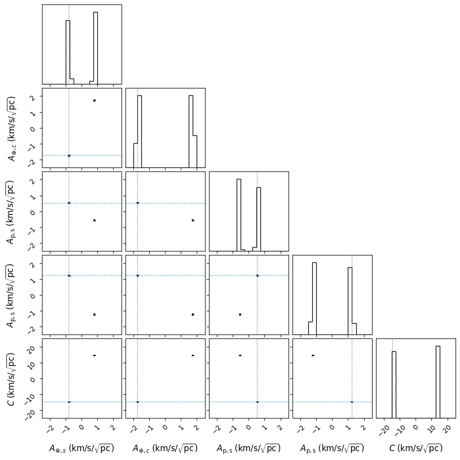
Visualize the samples, plotting only a small fraction, because the points are very bunched up at the zoomed-out scale that shows both solutions.

ranges_harc = [
    (-2.5, 2.5),
    (-2.5, 2.5),
    (-2.5, 2.5),
    (-2.5, 2.5),
    (-25., 25.),
]

fig = corner.corner(samp_harc_all[::400, :], labels=labels_harc,
                    range=ranges_harc, plot_contours=False, plot_density=False,
                    **corner_kwargs)

corner.core.overplot_lines(fig, truths_harc_list, lw=1, ls=':')

fig.set_size_inches(figsize_inches)

plt.show()

Select the samples that belong to one of the two solutions.

indices = (sol_sign.distribution == sol_sign_choice)

samp_harc_sel = samp_harc_all[indices, :]

display_samp_quantiles(samp_harc_sel, par_strs_harc, '.3f')

\[\begin{split}\displaystyle \begin{align}A_{\oplus,s} &= -0.803 \pm 0.028 \; \mathrm{km/s/\sqrt{pc}} \\[0.5em]A_{\oplus,c} &= -1.732 \pm 0.028 \; \mathrm{km/s/\sqrt{pc}} \\[0.5em]A_\mathrm{p,s} &= 0.547_{-0.027}^{+0.028} \; \mathrm{km/s/\sqrt{pc}} \\[0.5em]A_\mathrm{p,s} &= 1.218_{-0.028}^{+0.029} \; \mathrm{km/s/\sqrt{pc}} \\[0.5em]C &= -14.675 \pm 0.020 \; \mathrm{km/s/\sqrt{pc}} \\[0.5em]\end{align}\end{split}\]

Linear error propagation

For the linear error propagation, we select one of the two possible solutions and set up the harmonic coefficients as correlated variables with uncertainties using the uncertainties.correlated_values() function.

upars_harc = correlated_values(sol_sign_choice * popt, pcov)

display_ufloats(upars_harc, par_strs_harc, '.3f')

\[\begin{split}\displaystyle \begin{align}A_{\oplus,s} &= -0.803 \pm 0.028 \; \mathrm{km/s/\sqrt{pc}} \\[0.5em]A_{\oplus,c} &= -1.732 \pm 0.028 \; \mathrm{km/s/\sqrt{pc}} \\[0.5em]A_\mathrm{p,s} &= 0.547 \pm 0.028 \; \mathrm{km/s/\sqrt{pc}} \\[0.5em]A_\mathrm{p,s} &= 1.219 \pm 0.029 \; \mathrm{km/s/\sqrt{pc}} \\[0.5em]C &= -14.675 \pm 0.020 \; \mathrm{km/s/\sqrt{pc}} \\[0.5em]\end{align}\end{split}\]

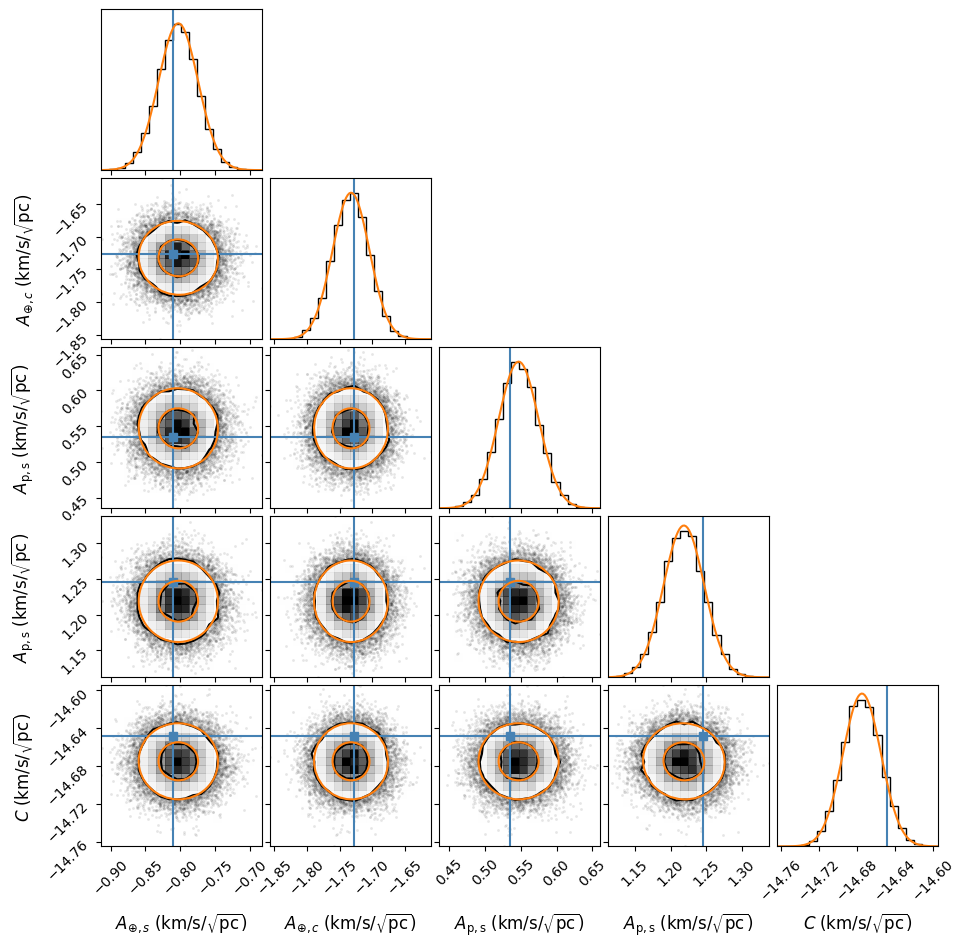
Visualize and compare the results of the two methods.

fig = corner.corner(samp_harc_sel, labels=labels_harc, truths=truths_harc_list,
                    labelpad=0.1, **corner_kwargs)

overplot_linear(fig, upars_harc, **linear_style)

fig.set_size_inches(figsize_inches)

plt.show()

The phenomenological parameters

While the primary reason for doing the error propagation described in this tutorial is usually to determine the uncertainties and correlations of the physical parameters, it may also be useful to check the constraints on the phenomenological parameters, which have a more straightforward relation to the data. In any case, the phenomenological parameters are an intermediate step in computing the physical parameters, and we may as well visualize the constraints at this step.

Monte Carlo sampling

Generate samples of the phenomenological model parameters. Then, to prepare the samples for plotting, combine the different free parameters into a single (unitless) NumPy array.

samp_phen = pars_harc2phen(samp_harc)

samp_phen_all = [dist.distribution.value for dist in samp_phen]
samp_phen_all = np.stack(samp_phen_all, axis=1)

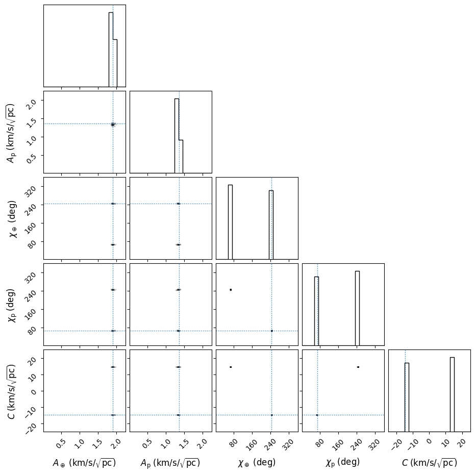
Visualize the samples, plotting only a small fraction, because the points are very bunched up at the zoomed-out scale that shows both solutions.

ranges_phen = [
    (0., 2.25),
    (0., 2.25),
    (0., 360.),
    (0., 360.),
    (-25., 25.),
]

fig = corner.corner(samp_phen_all[::400, :], labels=labels_phen,
                    range=ranges_phen, plot_contours=False, plot_density=False,
                    **corner_kwargs)

corner.core.overplot_lines(fig, truths_phen_list, lw=1, ls=':')

fig.set_size_inches(figsize_inches)

plt.show()

Filter the samples to select only the solution of choice.

indices = (sol_sign.distribution == sol_sign_choice)

samp_phen_sel = samp_phen_all[indices, :]

fmts_phen = ['.3f', '.3f', '.2f', '.1f', '.3f']
display_samp_quantiles(samp_phen_sel, par_strs_phen, fmts_phen)

\[\begin{split}\displaystyle \begin{align}A_\oplus &= 1.910_{-0.027}^{+0.028} \; \mathrm{km/s/\sqrt{pc}} \\[0.5em]A_\mathrm{p} &= 1.336 \pm 0.028 \; \mathrm{km/s/\sqrt{pc}} \\[0.5em]\chi_\oplus &= 245.13 \pm 0.85 \; \mathrm{deg} \\[0.5em]\chi_\mathrm{p} &= 65.8 \pm 1.2 \; \mathrm{deg} \\[0.5em]C &= -14.675 \pm 0.020 \; \mathrm{km/s/\sqrt{pc}} \\[0.5em]\end{align}\end{split}\]

Linear error propagation

Compute the phenomenological parameters using functions from the uncertainties.umath module.

upars_phen = upars_harc2phen(upars_harc)

display_ufloats(upars_phen, par_strs_phen, fmts_phen)

\[\begin{split}\displaystyle \begin{align}A_\oplus &= 1.909 \pm 0.028 \; \mathrm{km/s/\sqrt{pc}} \\[0.5em]A_\mathrm{p} &= 1.336 \pm 0.028 \; \mathrm{km/s/\sqrt{pc}} \\[0.5em]\chi_\oplus &= 245.14 \pm 0.86 \; \mathrm{deg} \\[0.5em]\chi_\mathrm{p} &= 65.8 \pm 1.2 \; \mathrm{deg} \\[0.5em]C &= -14.675 \pm 0.020 \; \mathrm{km/s/\sqrt{pc}} \\[0.5em]\end{align}\end{split}\]

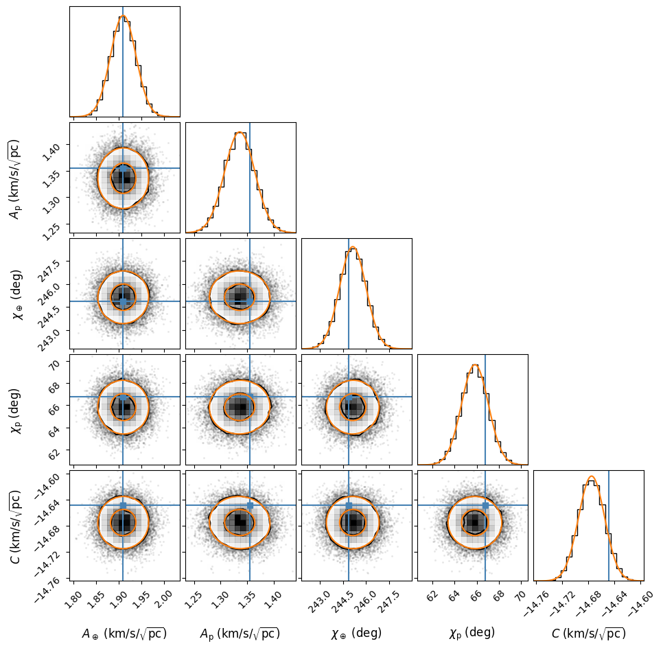
Visualize and compare the results of the two methods.

fig = corner.corner(samp_phen_sel, labels=labels_phen, truths=truths_phen_list,
                    labelpad=0.1, **corner_kwargs)

overplot_linear(fig, upars_phen, **linear_style)

fig.set_size_inches(figsize_inches)

plt.show()

The physical parameters

Because there are six physical parameters while the fitting only provides five constraints, external constraints need to be provided for one of the physical parameters to get narrow constraints on the rest. In this tutorial, we use a constraint on the pulsar distance \(d_\mathrm{p}\), which would also exist in many real-life applications. In the case of external constraints on a different parameter, the functions pars_phen2phys_d_p() and upars_phen2phys_d_p() defined above would have to be replaced with slightly different functions to convert from phenomenological to physical parameters.

The pulsar studied in this example, PSR J0437–4715, has an exceptionally well constrained distance of \(d_\mathrm{p} \approx 156.79 \pm 0.25\) pc. In this tutorial, however, we will instead use an artificial distance estimate with a much larger uncertainty of 30%, which is typical for a distance estimate derived from a pulsar’s dispersion measure using a model for the Galactic distribution of free electrons. This is done to make the example more similar to real-life applications (since most pulsars don’t have very precise distance estimates, but will have a known dispersion measure).

We now set the nominal value of the pulsar distance and its uncertainty, assumed to be Gaussian. The nominal value is different from the known pulsar distance of 157 pc to reflect measurement error. Note that the assumption of a normally distributed measurement error gives non-zero probabilities for zero and negative distances, which is unphysical. We will need to take care below to prevent this behaviour from causing problems.

d_p_mu = 200. * u.pc
d_p_sig = 60. * u.pc

Monte Carlo sampling

Generate a set of samples of the pulsar distance following a Gaussian distribution with the given mean and standard deviation. Redo samples with an unphysical non-positive distance. Finally, convert the set into an Astropy Distribution object.

d_p_iter = np.random.normal(size=nmc) * d_p_sig + d_p_mu

while np.any(d_p_iter <= 0):
    ind_neg = np.where(d_p_iter <= 0)
    d_p_replace = np.random.normal(size=len(ind_neg[0])) * d_p_sig + d_p_mu
    d_p_iter[ind_neg] = d_p_replace

samp_d_p = unc.Distribution(d_p_iter)

Generate random signs of the cosine of the pulsar’s orbital inclination, corresponding to the two possible spatial orientations of the pulsar’s orbit. We create an Astropy Distribution object consisting of +1 and -1 entries, just like sol_sign above.

rnd_sign = np.random.randint(low=0, high=2, size=nmc) * 2 - 1
cos_sign = unc.Distribution(rnd_sign)

Convert phenomenological to physical parameters and put the samples in a single array for the plotting routine.

samp_phys = pars_phen2phys_d_p(samp_phen, samp_d_p, cos_sign)

samp_phys_all = [dist.distribution.value for dist in samp_phys]
samp_phys_all = np.stack(samp_phys_all, axis=1)

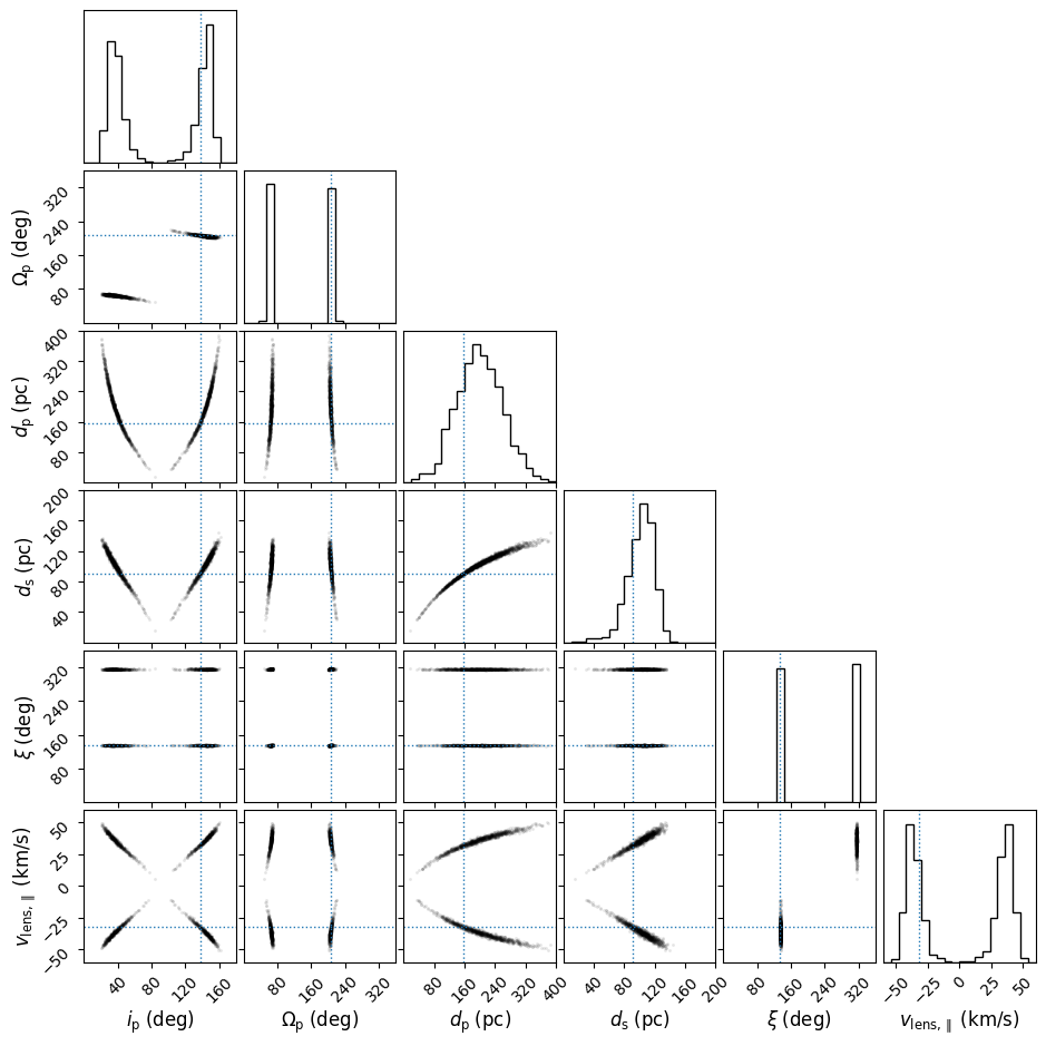
Visualize the samples, showing the different solutions. Again, only plot a small fraction of the samples, because of the overlap of the points.

ranges_phys = [
    (0., 180.),
    (0., 360.),
    (0., 400.),
    (0., 200.),
    (0., 360.),
    (-60., 60.),
]

fig = corner.corner(samp_phys_all[::20, :], labels=labels_phys,
                    range=ranges_phys, plot_contours=False, plot_density=False,
                    **corner_kwargs)

corner.core.overplot_lines(fig, truths_phys_list, lw=1, ls=':')

fig.set_size_inches(figsize_inches)

plt.show()

Filter the samples to select only the solution of choice.

cos_sign_choice = -1

indices = ((sol_sign.distribution == sol_sign_choice) &
           (cos_sign.distribution == cos_sign_choice))

samp_phys_sel = samp_phys_all[indices, :]

fmts_phys = ['.0f', '.1f', '.0f', '.0f', '.2f', '.1f']
display_samp_quantiles(samp_phys_sel, par_strs_phys, fmts_phys)

\[\begin{split}\displaystyle \begin{align}i_\mathrm{p} &= 144_{-11}^{+7} \; \mathrm{deg} \\[0.5em]\Omega_\mathrm{p} &= 205.1_{-2.1}^{+3.0} \; \mathrm{deg} \\[0.5em]d_\mathrm{p} &= 199_{-60}^{+61} \; \mathrm{pc} \\[0.5em]d_\mathrm{s} &= 103_{-19}^{+14} \; \mathrm{pc} \\[0.5em]\xi &= 134.86_{-0.82}^{+0.80} \; \mathrm{deg} \\[0.5em]v_\mathrm{lens,\parallel} &= -36.7_{-5.2}^{+6.8} \; \mathrm{km/s} \\[0.5em]\end{align}\end{split}\]

Linear error propagation

Set up the pulsar distance as a value with uncertainty using the uncertainties.ufloat() function.

ud_p = ufloat(d_p_mu.to_value(u.pc), d_p_sig.to_value(u.pc))

Compute the physical parameters using functions from the uncertainties.umath module.

upars_phys = upars_phen2phys_d_p(upars_phen, ud_p, cos_sign_choice)

display_ufloats(upars_phys, par_strs_phys, fmts_phys)

\[\begin{split}\displaystyle \begin{align}i_\mathrm{p} &= 144 \pm 9 \; \mathrm{deg} \\[0.5em]\Omega_\mathrm{p} &= 204.9 \pm 2.4 \; \mathrm{deg} \\[0.5em]d_\mathrm{p} &= 200 \pm 60 \; \mathrm{pc} \\[0.5em]d_\mathrm{s} &= 103 \pm 16 \; \mathrm{pc} \\[0.5em]\xi &= 134.86 \pm 0.82 \; \mathrm{deg} \\[0.5em]v_\mathrm{lens,\parallel} &= -36.8 \pm 5.8 \; \mathrm{km/s} \\[0.5em]\end{align}\end{split}\]

Visualize and compare the results of the two methods. For for the pulsar distance, we can also show the prior probability distribution to emphasize that this parameter was not retrieved by fitting the scintillation measurements, but inserted as an external constraint.

fig = corner.corner(samp_phys_sel, labels=labels_phys, truths=truths_phys_list,
                    labelpad=0.1, **corner_kwargs)

overplot_linear(fig, upars_phys, **linear_style)

ndim_phys = 6
idim_d_p = 2
npoints = 100

axes = np.array(fig.axes).reshape((ndim_phys, ndim_phys))

# d_p prior
ax = axes[idim_d_p, idim_d_p]
xlims = ax.get_xlim()

d_p_all = np.linspace(xlims[0], xlims[1], npoints) * u.pc
d_p_prior = st.norm.pdf(d_p_all.to_value(u.pc),
                        d_p_mu.to_value(u.pc),
                        d_p_sig.to_value(u.pc))

ax.plot(d_p_all.to_value(u.pc), d_p_prior, '--', color='C2')

fig.set_size_inches(figsize_inches)

fig.set_size_inches(figsize_inches)

plt.show()

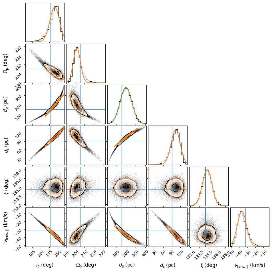
This final figure illustrates that the linear error propagation is unable to capture the nonlinearities (curves) in the correlations between parameters, as well as the asymmetries in the probability density distributions of some of the parameters. The plot also shows that the constraints on all physical parameters (except for the screen angle \(\xi\)) strongly depend on how well the pulsar’s distance \(d_\mathrm{p}\) is known.